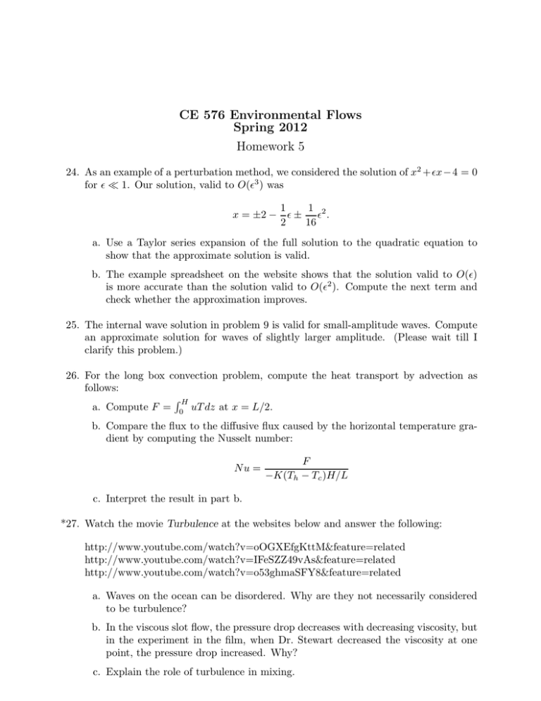
CE 576 Environmental Flows
Spring 2012
Homework 5
24. As an example of a perturbation method, we considered the solution of x2 +x −4 = 0
for 1. Our solution, valid to O(3 ) was
1
1
x = ±2 − ± 2 .
2
16
a. Use a Taylor series expansion of the full solution to the quadratic equation to
show that the approximate solution is valid.
b. The example spreadsheet on the website shows that the solution valid to O()
is more accurate than the solution valid to O(2 ). Compute the next term and
check whether the approximation improves.
25. The internal wave solution in problem 9 is valid for small-amplitude waves. Compute
an approximate solution for waves of slightly larger amplitude. (Please wait till I
clarify this problem.)
26. For the long box convection problem, compute the heat transport by advection as
follows:
H
a. Compute F = 0 uT dz at x = L/2.
b. Compare the flux to the diffusive flux caused by the horizontal temperature gradient by computing the Nusselt number:
Nu =
F
−K(Th − Tc )H/L
c. Interpret the result in part b.
*27. Watch the movie Turbulence at the websites below and answer the following:
http://www.youtube.com/watch?v=oOGXEfgKttM&feature=related
http://www.youtube.com/watch?v=IFeSZZ49vAs&feature=related
http://www.youtube.com/watch?v=o53ghmaSFY8&feature=related
a. Waves on the ocean can be disordered. Why are they not necessarily considered
to be turbulence?
b. In the viscous slot flow, the pressure drop decreases with decreasing viscosity, but
in the experiment in the film, when Dr. Stewart decreased the viscosity at one
point, the pressure drop increased. Why?
c. Explain the role of turbulence in mixing.
d. In the example of the two jets at different Reynolds numbers, the Reynolds number does not determine the large scales of the flow. What does?
e. Which movie scene was fake?
f. Explain how density stratification reduces mixing.
g. What was your favorite part of the movie? Why?
*28. Find an example of a turbulent flow either in a picture or in the Ames area. Provide
a copy of the picture or a description of its location. Argue that the flow is turbulent
by discussing it in terms of the characteristics (i.e., disorder, mixing, wide range of
eddies, high Reynolds number) we identified in class.
*29. We showed that the depth-averaged velocity in a channel with a logarithmic velocity
profile is
H
0.4H
u∗
u∗
ln
ln
U=
≈
,
κ
ey0
κ
y0
where u∗ is the shear velocity, κ = 0.4 is von Kármán’s coefficient, H is the water
depth, and y0 is the roughness length. This relation is the basis for streamflow measurements of the U.S. Geological Survey: When the profile is logarithmic, the mean
velocity occurs at y = 0.4H, with y measured from the channel bottom. An alternative approach is to measure the velocities at y = 0.2H and y = 0.8H and average
them. Show that this approach yields the depth-averaged velocity.