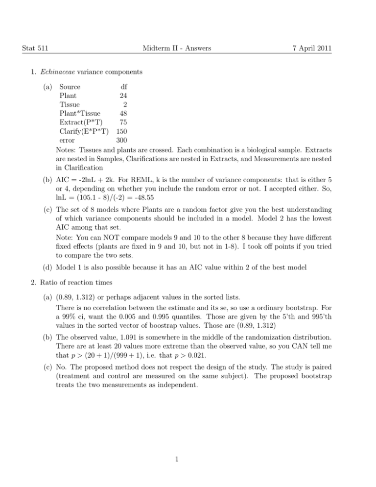
Stat 511
Midterm II - Answers
7 April 2011
1. Echinaceae variance components
(a) Source
df
Plant
24
Tissue
2
Plant*Tissue
48
Extract(P*T)
75
Clarify(E*P*T) 150
error
300
Notes: Tissues and plants are crossed. Each combination is a biological sample. Extracts
are nested in Samples, Clarifications are nested in Extracts, and Measurements are nested
in Clarification
(b) AIC = -2lnL + 2k. For REML, k is the number of variance components: that is either 5
or 4, depending on whether you include the random error or not. I accepted either. So,
lnL = (105.1 - 8)/(-2) = -48.55
(c) The set of 8 models where Plants are a random factor give you the best understanding
of which variance components should be included in a model. Model 2 has the lowest
AIC among that set.
Note: You can NOT compare models 9 and 10 to the other 8 because they have different
fixed effects (plants are fixed in 9 and 10, but not in 1-8). I took off points if you tried
to compare the two sets.
(d) Model 1 is also possible because it has an AIC value within 2 of the best model
2. Ratio of reaction times
(a) (0.89, 1.312) or perhaps adjacent values in the sorted lists.
There is no correlation between the estimate and its se, so use a ordinary bootstrap. For
a 99% ci, want the 0.005 and 0.995 quantiles. Those are given by the 5’th and 995’th
values in the sorted vector of boostrap values. Those are (0.89, 1.312)
(b) The observed value, 1.091 is somewhere in the middle of the randomization distribution.
There are at least 20 values more extreme than the observed value, so you CAN tell me
that p > (20 + 1)/(999 + 1), i.e. that p > 0.021.
(c) No. The proposed method does not respect the design of the study. The study is paired
(treatment and control are measured on the same subject). The proposed bootstrap
treats the two measurements as independent.
1
Stat 511
Midterm II - Answers
7 April 2011
3. Reaction times, part 2
(a) There are 80 df in the table, so there are 119-80 = 39 missing observations
There are 1+2+2+41 = 46 df for the main plot (subjects) part of the ANOVA table (sex
+ age + sex*age + subject(sex*age)). So there are 59 - 46 = 13 missing subjects.
Notes: A lot of folks missed the second part because they computed 59 - subject(sex*age).
That ignores the additional df associated with groups (treatments) of subjects.
(b)






1
0
0
0
0
0
1
1
0
0
0
0
0
1
1






Notes: there are three subjects included in this snippet of data: two 60yr old males and
one 18yr old female. The first subject has 1 obs., the other two provide 2 obs.
(c) Σ = ZGZ 0 + R =






2
0
0
0
0
+ σs2
σm
2
2
2
0
0
σm
0
σm + σs
2
2
0
σm
σm
+ σs2
0
0
2
2
2
0
0
0
σm + σs
σm
2
2
σm + σs2
0
0
0
σm






2
= 1.92
(d) σ̂m
MS for error = 1.30 = σ̂s2
2
MS for subjects = 4.53 = 1.30 + 1.683 σm
2
σ̂m = (4.53 − 1.30)/1.683 = 1.92
(e) F = MS(trt*age) / MS (error) = 3.508 / 1.297 = 2.7
Notes: MS for Trt*Age = 7.016/2 = 3.508. The appropriate denominator is MS error
= 36.327/28 = 1.297. You can see this either by reasoning that trt*age is a split plot or
within-subject factor or by noticing that the E MS for trt*age only include σe2
(f) No need for C-S. numerator 2 df, denominator 28 df.
2
(g) The MS for sex = 4.157/1 = 4.157. The appropriate denominator is σs2 + 1.529σm
. This
2
2
can be calculated either by plugging in the estimates σ̂s and σ̂m to get 1.30 + 1.529× 1.92
= 4.24, or by figuring out that E 0.9085M Ssubject(sex∗age) + 0.0915M Serror = M Serror +
1.529M Ssubject(sex∗age) . If you use the latter approach, you get the same denominator
MS: 0.9085*4.53 + 0.0915 * 1.30 = 4.23. Hence, F = 4.157 / 4.23 = 0.98
2
Stat 511
Midterm II - Answers
7 April 2011
(h) numerator df = 1. denominator df requires C-S: The MS used as the denominator is
0.908 M Sm + 0.092 M Ss . The C-S calculations are:
X
ai M Si = 4.24 Note: already have this #
X
0.9082 4.532 0.0922 1.302
2
2
ai M Si /dfi =
+
41
28
= 0.413 + 0.001
= 0.413
νcs = 4.242 /0.413
= 43.51
There are many opportunities for rounding errors that lead to slightly different answers.
Anything close to this and derived in a reasonable way was accepted.
4. Curvature of wings
(a) Source
df
Curvature
2
Wing(Curv.) 3
subsampling 54
.̧total
59
Explanation: You are told that the curvature is randomly assigned to a wing. So wings
are the eu. There are 6 of these. Wings are nested within curvature levels; a single wing
has one and only one curvature. The 10 observations made on each wing are subsamples.
If you wrote out a model, the ANOVA table above corresponds to
Yijk = µ + αi + ωij + ijk
2
ωij ∼ N (0, σwing
2
ijk ∼ N (0, σobs
where i indexes curvature level, j indexes wing, and k indexes observation. The E MS
for this model are
Source
E MS
2
2
Curvature
σobs
+ 10σwing
+ Q(curvature)
2
2
Wing(Curv.) σobs + 10σwing
2
subsampling σobs
(b) Wing(curv.) is the appropriate denominator for to test differences among curvatures.
This follows from the ’use the eu variability to test effects assigned to eu’s. Or, it follows
directly from the E MS for subsampling.
3
Stat 511
Midterm II - Answers
7 April 2011
5. Biorenewables
(a) Source
df
Expt
2
Block(Expt.) 12
Temp
2
Expt*Temp
4
w/i Expt
24
.̧total
59
I also accepted for full credit the model with blocks crossed with experiments, i.e.
Source
df
Expt
2
Block
4
Expt*Block
8
Temp
2
Expt*Temp 4
w/i Expt
24
.̧total
59
Explanation: This is a repeated experiment. Each of the three experiments is an RCBD.
The experiments are likely to give different (perhaps only slightly different) results because each experiment uses a different batch of corn stalks. All the eu’s within experiment
1 use the same batch of corn stalks. I tell you that batches of corn stalks have different
composition.
Experiment*Temp is included because we are concerned about the consistency of the
treatment effects across experiments.
Other common answers that got partial credit (some more than others) and why they
are not appropriate:
RCBD with only blocks, no mention of experiment: does not separate the variability between experiments from the variability within an experiment (the w/i Expt =
block(expt)*temp error)
Some form of split plot design with experiment as the split plot factor: You could view
this as a split plot with corn stalk batch = experiment “assigned” to a main plot eu that
is not replicated. Temp is clearly assigned to a smaller size eu. If you want to think of
this as a split plot design, temp is the split factor, not experiment.
Only 2 df for blocks: I presume you misread the picture and thought there were 3 blocks,
instead of 5.
(b) If we want broad sense inference, expt*temp is the appropriate error for temp.
I gave partial credit to block*temp. The residual got no credit (that would be narrow
sense inference).
4