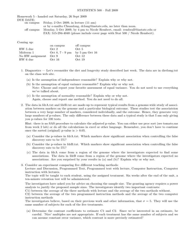
STATISTICS 500 – Fall 2009
Homework 5 - handed out Saturday, 26 Sept 2009
DUE DATE:
on campus Friday, 2 Oct 2009, in lecture (11 am)
or by e-mailto Chuanlong, dclong@iastate.edu, no later than noon.
off campus Monday, 5 Oct 2009, by 4 pm to Nicole Rembert, email: rembeall@iastate.edu or
FAX: 515-294-4040 (please include cover page with Stat 500 / Nicole Rembert).
Coming up:
HW 5 due
Midterm 1
No HW assignment
HW 6 due
on campus
Oct 2
Oct 8, 7 - 9 pm
Oct 9
Oct 16
off campus
Oct 5
by 5 pm Oct 16
Oct 12
Oct 19
1. Diagnostics — Let’s reconsider the diet and longevity study described last week. The data are in dietlong.txt
on the class web site.
(a) Is the assumption of independence reasonable? Explain why or why not.
(b) Is the assumption of equal variance reasonable? Explain why or why not.
Note: Choose and report your favorite assessment of equal variance. You do not need to use everything
we’ve talked about.
(c) Is the assumption of normality reasonable? Explain why or why not.
Again, choose and report one method. You do not need to do all.
2. The data in fdrA.txt and fdrB.txt are made-up to represent typical results from a genome-wide study of association between markers on the genome and a particular biological outcome. These studies test the associateion
between a very large number of markers, considered individually, and the outcome. Hence, they generate very
large numbers of p-values. The only difference between these data and a typical study is that I am only giving
you p-values for 100 tests.
Hint: there is no SAS procedure to calculate the adjusted p-value. You can either use proc sort (see tomato.sas
from week 2 lab) or do all the calculations in excel or other language. Remember, you don’t have to continue
once the sorted (original) p-value is > 0.05.
(a) Consider the p-values in fdrA.txt. Which markers show significant association when controlling the false
discovery rate to be 5%?
(b) Consider the p-values in fdrB.txt. Which markers show significant association when controlling the false
discovery rate to be 5%?
(c) The data in fdrA come from a region of the genome where the investigators expected to find some
associations. The data in fdrB come from a region of the genome where the investigators expected no
associations. Are you surprised by your results in (a) and (b)? Explain why or why not.
3. Consider an experiment comparing five different teaching methods:
Lecture and Discussion, Programmed Text, Programmed text with lecture, Computer Instruction, Computer
instruction with lectures.
The topic will be taught to each student, using the assigned treatment. Six weeks after the end of the unit, a
ten-minute retention test will be administered.
The investigators have asked you for advice on choosing the sample size. The granting agency requires a power
analysis to justify the proposed sample sizes. The investigators identify two important contrasts:
C1) between the average of the three methods with lecture and the average of the two methods without.
C2) between the average of the two programmed instruction methods and the average of the two computer
instruction methods
The investigators believe, based on their previous work and other information, that σ = 5. They will use the
same number of subjects for each of the five treatments.
(a) Determine the contrast coefficients to estimate C1 and C2. Since we’re interested in an estimate, be
careful. ’Nice’ multiples are not appropriate. If each treatment has the same number of subjects and we
can assume constant error variance, which contrast is more precisely estimated?
(b) The investigators decide to base the sample size determination on C1, because it is slightly more important
than C2. They are interested in a difference of 3 units. Assume a two-sided test with α = 5%. If all
treatments have the same sample size, what number of subjects per treatment, n, is needed for 80% power?
(c) The investigators can use a maximum of 60 subjects. C1 is still the most important contrast, so the
investigators want to estimate this as precisely as possible. Assume all treatments have the same variance.
Would it be better to use a design with:
D1) 12 subjects per treatment, or
D2) 10 subjects in each of the 3 treatments with lectures (L+D, R+L, C+L) and 15 subjects in both of
the treatments without lectures (R, C)?
Note: you do not need to calculate power for either design.
4. Analysis of paired data —
The data in platelet.txt are from a study of the physiological effects of smoking. The subjects are 11 nonsmokers. The response is the extent of platelet aggregation. Aggregation normally happens at the site of a cut.
That’s what forms the scab. Platelet aggregation inside blood vessels is bad. That increases the probability of
heart attacks.
In this study, blood was drawn and platelet aggregation measured. Then the subject smoked a cigarette. Thirty
minutes later, blood was again drawn and platelet aggregation measured. There are two responses for each
subject (before and after).
(a) Estimate the mean difference between before and after smoking. Use t quantiles to estimate a 95%
confidence interval for the difference.
(b) Use a paired t-test to test the hypothesis of no difference.
(c) Is the paired t-test appropriate here?
Note: I’m not asking about a paired t-test vs. a two sample t-test.
(d) Find the variance among the before observations and the variance among after observations. Use these to
calculate the variance of the mean difference if you ignored the pairing. (you may use the unequal variance
formula or compute s2p then use the equal variance formula). Compare this to the correct variance of the
mean difference. Is a paired design a good idea for this sort of experiment? Explain why or why not.
(e) The data in platelet2.txt are the same data organized in a form that is easy to use in an ANOVA with
blocks. Each row is now a single observation and there is a new variable, subject, that is used to identify
the blocks.
Analyze the data using a RCBD model. Do you get the same p-value for the test of no effect of smoking
as you did in the paired t-test?
5. Analysis of data from a block design – Fat in Diets
The data in dietfat.txt were collected in a study of the impact of diet on blood lipid levels. In general, high
blood lipid levels indicate a higher risk of heart attack. In this study, 15 men were grouped by age into five
groups with 3 subjects per group. Within each group, three diets (EL: extremely low in fat, FL: fairly low, and
ML: moderately low) were randomly assigned to the three men in each age group. The response is the change
in lipid level after 3 weeks on the diet.
(a) Assume that the standard assumptions hold and test the hypothesis of no differences among diets. Report
your test statistic, p-value, and a 1-sentence conclusion.
(b) The invesigators are especially interested in whether there is a difference between the extremely low and
fairly low diets. This was the primary question to be answered by the study. Estimate this difference
and a 95% confidence interval. Test whether the null hypothesis of no difference, adjusting for multiple
comparisons if appropriate.
(c) Calculate the efficiency of blocking.
(d) If the investigators repeat their study, would you recommend that they block by age?