STATISTICS 402B
Spring 2016
Homework Set#5 Solution
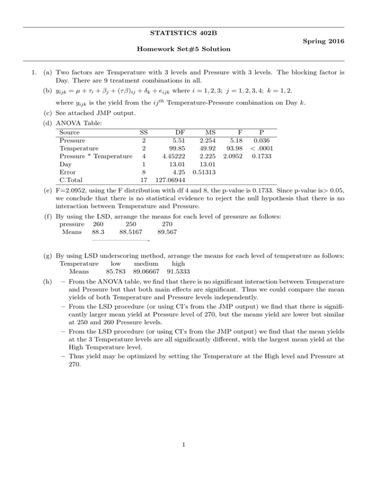
1. (a) Two factors are Temperature with 3 levels and Pressure with 3 levels. The blocking factor is
Day. There are 9 treatment combinations in all.
(b) yijk = µ + τi + βj + (τ β)ij + δk + eijk where i = 1, 2, 3; j = 1, 2, 3, 4; k = 1, 2.
where yijk is the yield from the ij th Temperature-Pressure combination on Day k.
(c) See attached JMP output.
(d) ANOVA Table:
Source
Pressure
Temperature
Pressure * Temperature
Day
Error
C.Total
SS
2
2
4
1
8
17
DF
5.51
99.85
4.45222
13.01
4.25
127.06944
MS
2.254
49.92
2.225
13.01
0.51313
F
5.18
93.98
2.0952
P
0.036
< .0001
0.1733
(e) F=2.0952, using the F distribution with df 4 and 8, the p-value is 0.1733. Since p-value is> 0.05,
we conclude that there is no statistical evidence to reject the null hypothesis that there is no
interaction between Temperature and Pressure.
(f) By using the LSD, arrange the means for each level of pressure as follows:
pressure 260
250
270
Means 88.3
88.5167
89.567
————————(g) By using LSD underscoring method, arrange the means for each level of temperature as follows:
Temperature
low
medium
high
Means
85.783 89.06667 91.5333
(h)
– From the ANOVA table, we find that there is no significant interaction between Temperature
and Pressure but that both main effects are significant. Thus we could compare the mean
yields of both Temperature and Pressure levels independently.
– From the LSD procedure (or using CI’s from the JMP output) we find that there is significantly larger mean yield at Pressure level of 270, but the means yield are lower but similar
at 250 and 260 Pressure levels.
– From the LSD procedure (or using CI’s from the JMP output) we find that the mean yields
at the 3 Temperature levels are all significantly different, with the largest mean yield at the
High Temperature level.
– Thus yield may be optimized by setting the Temperature at the High level and Pressure at
270.
1
JMP Analysis of Problem 5.1 Homework Set#5
Analysis of Variance
Source
DF
Model
Error
C. Total
9
8
17
Sum of
Squares
122.81944
4.25000
127.06944
Mean Square
F Ratio
13.6466
0.5313
25.6877
Prob > F
<.0001*
Effect Tests
Source
DF
Pressure
Temperature
Pressure*Temperature
Day
2
2
4
1
Sum of
Squares
5.507778
99.854444
4.452222
13.005000
F Ratio
5.1838
93.9807
2.0952
24.4800
Prob >
F
0.0360*
<.0001*
0.1733
0.0011*
Effect Details
Pressure
Least Squares Means Table
Level
250
260
270
Least Sq
Mean
88.516667
88.300000
89.566667
Std Error
Mean
0.29755952
0.29755952
0.29755952
88.5167
88.3000
89.5667
LSMeans Differences Student's t
α=
0.050
t=
2.306
LSMean[i] By LSMean[j]
Mean[i]-Mean[j]
250
260
Std Err Dif
Lower CL Dif
Upper CL Dif
250
0 0.21667
0 0.42081
0 -0.7537
0 1.18706
260
-0.2167
0
0.42081
0
-1.1871
0
0.75373
0
270
1.05 1.26667
0.42081 0.42081
0.0796 0.29627
2.0204 2.23706
Level
270 A
250
B
260
B
Temperature
Least Squares Means Table
Level
Least Sq Mean
Std Error Mean
Low
85.783333 0.29755952 85.7833
Medium
89.066667 0.29755952 89.0667
High
91.533333 0.29755952 91.5333
LSMeans Differences Student's t
270
-1.05
0.42081
-2.0204
-0.0796
-1.2667
0.42081
-2.2371
-0.2963
0
0
0
0
Least Sq Mean
89.566667
88.516667
88.300000
Levels not connected by same letter are significantly
different.
α=
0.050
t=
2.306
LSMean[i] By LSMean[j]
Mean[i]-Mean[j]
Low Medium
Std Err Dif
Lower CL Dif
Upper CL Dif
Low
0 -3.2833
0 0.42081
0 -4.2537
0 -2.3129
Medium
3.28333
0
0.42081
0
2.31294
0
4.25373
0
High
5.75 2.46667
0.42081 0.42081
4.7796 1.49627
6.7204 3.43706
Level
High
A
Medium
B
Low
C
High
-5.75
0.42081
-6.7204
-4.7796
-2.4667
0.42081
-3.4371
-1.4963
0
0
0
0
Least Sq Mean
91.533333
89.066667
85.783333
Levels not connected by same letter are significantly
different.
Problem 2
(a)
1
 = 2×6
(223 + 192 − 156 − 140) = 119
12 = 9.9167
1
−15
B̂ = 2×6 (156 + 192 − 223 − 140) = 12 = −1.25
ˆ = 1 (192 + 140 − 223 − 156) = −47 = −3.9167
AB
2×6
12
(b)
(c)
See JMP output
(d)
SSA = 1192 /24 = 590.04167
SSAB = (−47)2 /24 = 92.04167
SST rt = SSA + SSB + SSAB = 691.45833
SSE = SST ot − SST rt = 793.63 − 691.458 = 102.17
SV
Time
Medium
T* M
Error
Total
DF
1
1
1
20
23
SS
590.04
9.38
92.04
102.17
793.63
MS
590.04
9.38
92.04
5.11
F
115.5
1.84
18.01
1
3. .
(a) ANOVA Table
Source of Variation
Treatment
Error
Total
d.f.
7
8
15
SS
153
23
176
(b),(c) Table of Contrast Values, Effects, and Sums of Squares
Treatment
Combination
(1)
a
b
ab
c
ac
bc
abc
Contrast
Divisor for Estimate
Estimate of Effect
Divisor for SS
SS of Effect
Observed
Total
8
11
15
22
15
9
25
23
I
+
+
+
+
+
+
+
+
16
16
A
+
+
+
+
2
8
0.25
16
0.25
B
+
+
+
+
42
8
5.25
16
110.25
Factorial Effect
AB
C
AC
+
+
+
+
+
+
+
+
+
+
+
+
8
16
-18
8
8
8
1.0
2.0
-2.25
16
16
16
4.0
16.0
20.25
BC
+
+
+
+
6
8
0.75
16
2.25
ABC
+
+
+
+
0
8
0
16
0
(d) ANOVA Table: Breakdown of Treatment SS
Source of Variation
A
B
AB
C
AC
BC
ABC
Error
Total
d.f.
SS
1 0.25
1 110.25
1
4.0
1 16.0
1 20.25
1 2.25
1
0.0
8 23.0
15 176.0
MS
0.25
110.25
4.0
16.0
20.25
2.25
0.0
2.875
F
0.087
38.348
1.391
5.565
7.043
0.783
0.0
p-value
.7756
.0003
.2721
.0460
.0291
.4021
1.0000
The p-values for main effect B, main effect C and interaction effect AC are less than .05; thus these
effects are significantly different from zero at α = .05
(e) .
I will use the tables of means and plots in the JMP output under Effect B and Effect A*C (in Effect
Details section)
Effect B: both the table and graph clearly shows that the Effect B is positive and increases the mean
yield by 5.25.
Effect A*C:
C
A
0
0
5.75
1
10.0
1
8.25
8.0
Both the above table and the graph indicates that Effect C is positive at the low level of A and not
significant at high level of A. At the low level of A, effect of C is to increase mean yield by 4.25
(f) .
For Factor B, a 95% CI for the difference µ0 − µ1 is (−7.205, −3.295)
For Interaction AC: 95% CI’s for the means of C at level 0 of A µ00 − µ01 is (−7.0148, −1.4852)
95% CI’s for the means of C at level 1 of A µ10 − µ11 is (−2.5148, 3.0148)
Level
1
A
0
B
Response Yield
Analysis of Variance
Source
DF
Model
Error
C. Total
7
8
15
Sum of
Squares
153.00000
23.00000
176.00000
Mean Square
F Ratio
21.8571
2.8750
7.6025
Prob > F
0.0052*
Levels not connected by same letter are significantly different.
A*C
Least Squares Means Table
Level
0,0
0,1
1,0
1,1
Effect Tests
Source DF Sum of Squares F Ratio Prob > F
A
1
0.25000 0.0870
0.7756
B
1
110.25000 38.3478 0.0003*
A*B
1
4.00000 1.3913
0.2721
C
1
16.00000 5.5652 0.0460*
A*C
1
20.25000 7.0435 0.0291*
B*C
1
2.25000 0.7826
0.4021
A*B*C
1
0.00000 0.0000
1.0000
Least Sq Mean
10.625000
5.375000
Least Sq
Mean
5.750000
10.000000
8.250000
8.000000
Std Error
0.84779125
0.84779125
0.84779125
0.84779125
LS Means Plot
Effect Details
B
Least Squares Means Table
Level
0
1
Least Sq
Mean
5.375000
10.625000
Std Error
Mean
0.59947894
0.59947894
5.3750
10.6250
LS Means Plot
LSMeans Differences Student's t
α=
0.050
t=
LSMean[i] By LSMean[j]
Mean[i]-Mean[j]
Std Err Dif
Lower CL Dif
Upper CL Dif
0
1
2.306
0
1
0
-5.25
0 0.84779
0
-7.205
0
-3.295
5.25
0
0.84779
0
3.29499
0
7.20501
0
LSMeans Differences Student's t
α=
0.050
t=
2.306
LSMean[i] By LSMean[j]
Mean[i]-Mean[j]
0,0
0,1
Std Err Dif
Lower CL Dif
Upper CL Dif
0,0
0
-4.25
0 1.19896
0 -7.0148
0 -1.4852
0,1
4.25
0
1.19896
0
1.4852
0
7.0148
0
1,0
2.5
-1.75
1.19896 1.19896
-0.2648 -4.5148
5.2648 1.0148
1,1
2.25
-2
1.19896 1.19896
-0.5148 -4.7648
5.0148 0.7648
Level
0,1
A
1,0
A B
1,1
A B
0,0
B
1,0
1,1
-2.5
1.19896
-5.2648
0.2648
1.75
1.19896
-1.0148
4.5148
0
0
0
0
-0.25
1.19896
-3.0148
2.5148
-2.25
1.19896
-5.0148
0.5148
2
1.19896
-0.7648
4.7648
0.25
1.19896
-2.5148
3.0148
0
0
0
0
Least Sq Mean
10.000000
8.250000
8.000000
5.750000
Levels not connected by same letter are significantly different.