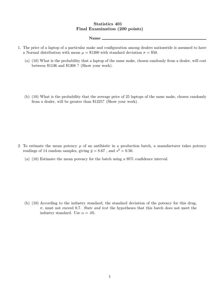
Statistics 401
Final Examination (200 points)
Name
1. The price of a laptop of a particular make and configuration among dealers nationwide is assumed to have
a Normal distribution with mean µ = $1200 with standard deviation σ = $50.
(a) (10) What is the probability that a laptop of the same make, chosen randomly from a dealer, will cost
between $1136 and $1308 ? (Show your work).
(b) (10) What is the probability that the average price of 25 laptops of the same make, chosen randomly
from a dealer, will be greater than $1225? (Show your work).
2. To estimate the mean potency µ of an antibiotic in a production batch, a manufacturer takes potency
readings of 14 random samples, giving ȳ = 8.67 , and s2 = 0.56.
(a) (10) Estimate the mean potency for the batch using a 95% confidence interval.
(b) (10) According to the industry standard, the standard deviation of the potency for this drug,
σ, must not exceed 0.7. State and test the hypotheses that this batch does not meet the
industry standard. Use α = .05.
1
3. Brands of a type of electrical wire produced by two different manufacturers are being studied to compare
their resistivity characteristics. The values of resistivity measurements obtained by the experimenter suggests that they can be considered to be samples from normal distributions and are used to calculate the
following statistics:
Brand A
Brand B
2
n1 = 8 ȳ1. = 0.140 s1 = 0.000007 n2 = 9 ȳ2. = 0.145 s22 = 0.00002
Assuming that the population means are µ1 and µ2 and the population variances are σ12 and σ22 , respectively,
answer the following questions:
(a) (10) Test the hypothesis H0 : σ12 = σ22 vs. Ha : σ12 6= σ22 . Use α = .05 and show work.
(b) (10) Now assume σ12 = σ22 . Compute the standard error of the difference in the sample means ȳ1. − ȳ2. .
(c) (10) Use the standard error from part (b) to construct a statistic to test the research hypothesis that
Brand B wires have larger mean resistivity. State the null and alternative, the rejection region, and
your decision using α = .05. Show work.
(d) (10) Use the standard error from part (b) to compute a 90% confidence interval for µ1 − µ2 . Test the
hypothesis in part (c) using this interval, stating the α-level of the test.
2
4. An experiment was conducted to determine the relationship between the amount of warping in thin strips,
(y), made from a particular alloy and temperature, (x) . A simple linear regression model of the form
y = β0 + β1 x + was first fitted to the data.
Temperature
(◦ C ) (x)
Amount of
Warping (y)
ȳi.
15
11, 11, 14
12
20
14, 12, 13
13
25
14, 12, 16
14
30
18, 14, 16
16
35
21, 19, 17
19
40
24, 20, 22
22
45
24, 23, 28
25
50
31, 30, 32
31
The following statistics have also been computed from the above data:
Sxx = 3150.0
Syy = 980.0
Sxy = 1650.0
(a) (10) Complete the analysis of variance table for the regression below. Use the F-ratio from the anova
table to test H0 : β1 = 0 vs. Ha : β1 6= 0, at α = .05. Show work and state your conclusion.
Source
d.f.
SS
MS
F
Regression
Error
Total
23
(b) (10) Compute the t-statistic to test the hypothesis that H0 : β1 = 0 vs. Ha : β1 6= 0. Test this
hypothesis using α = .05. State the rejection region and your decision clearly. Show work.
3
(c) (10) Perform the lack of fit test by completing the following table and state your conclusion. Use
α = .05.
d.f.
Source
SS
MS
F
Lack of Fit
Pure Error
Total Error
(d) (10) Based on the above analysis and examining relevant residual plots, it was decided to fit
the polynomial model y = β0 + β1 x + β2 x2 + to this data. Using the JMP output of this
fit given below, test the hypothesis that the squared term is necessary in this model. Use
α = .05. State the null and alternative hypotheses, circle the test statistic and the
p-value, and state your conclusion.
Term
Intercept
x
x*x
Estimate
14.309524
-0.342857
0.0133333
Std Error t-Ratio
2.965769
4.82
0.197591
-1.74
0.003005
4.44
Prob>|t|
<.0001
0.0974
0.0002
5. In a laboratory experiment, the weight loss in milligrams of a certain machine part due to friction when
specimens were used in a wear-tester with four different lubricants SP51, L43, Z907, and Blu-Tek, were
measured. Lower the weight loss, the better the performance of the lubricant. The lubricants were assigned
to the test runs completely at random. The model yij = µi + ij , i = 1, . . . , 4; j = 1, . . . , 8 with ij ∼
N (0, σ2 ), was used to analyze the resulting data:
i
1
2
3
4
Lubricant
SP51
L43
Z907
Blu-Tek
12
8
10
8
11
10
5
5
Weight Loss (in milligrams)
7
10
9
10
5
7
10
9
7
8
9
6
8
7
5
6
12
7
7
6
7
8
6
7
ȳi.
9.75
8.0
7.25
6.5
(a) (10) Complete the analysis of variance table below by filling in the blanks. State the null and
alternative hypotheses you test using the F-ratio. Perform this test using α = .05.
Source
Lubricant
d.f.
SS
46.5
MS
Error
Total
123.5
4
F
(b) (10) Sp51 and L43 are petroleum distillate based lubricants while Z907 and Blu-Tek are synthetic
oil based lubricants. Is the average performance of the petroleum distillate based lubricants same as
the average performance of the synthetic oil based lubricants? To answer this question, calculate a
t-statistic to test the hypothesis H0 : (µ1 + µ2 )/2 = (µ3 + µ4 )/2 vs. Ha : (µ1 + µ2 )/2 6= (µ3 + µ4 )/2
State your conclusion using α = .05?
(c) (10) Sp51 and Z907 contain a standard silicon additive while L43 and Blu-Tek contain a new hi-tech
detergent additive. Is the new additive result in better performance in the detergents than when
using the standard additive? To answer this question, calculate a t-statistic to test the hypothesis
H0 : (µ1 + µ3 )/2 ≤ (µ2 + µ4 )/2 vs. Ha : (µ1 + µ3 )/2 > (µ2 + µ4 )/2
State your conclusion using α = .05?
(d) (10) Compute the LSD value at α = .05. Use the LSD multiple comparison procedure to compare the
4 lubricant means using the underlining method. Summarize the results of this procedure in words.
5
6. The data below, extracted from Consumer Reports, comprise of gasoline mileage, y, measured as gallons
per 100 miles (GP100M), and six aspects of automobile design and performance for 36 automobiles in a
certain model year. It is desired to develop a regression model to predict gasoline mileage of a vehicle using
6 explanatory variables measured: CYL=Number of Cylinders, DISP= Engine Size in cubic inches, HP=
Horsepower, DRAT=Drive Ratio, WT=Weight in lbs., ACCEL= Acceleration in sec.
Automobile
Ford Country Sq.
Chevy Malibu Wag
Chevette
Toyota Corona
Datsun 510
Dodge Omni
Audi 5000
Volvo 240 GL
Saab 99 GLE
Peugeot 694 SL
Buick Century Sp
Mercury Zephyr
Dodge Aspen
AMC Concord D/L
Chevy Caprice Cl
Ford LTD
Mercury Grand Ma
Dodge St Regis
Ford Mustang 4
Ford Mustang Ghi
Mazda GLC
Dodge Colt
AMC Spirit
VW Scirocco
Honda Accord LX
Buick Skylark
Chevy Citation
Olds Omega
Pontiac Phoenix
Plymouth Horizon
Datsun 210
Fiat Strada
VW Dasher
Datsun 810
BMW 320i
VW Rabbit
CYL
8
8
4
4
4
4
5
6
4
6
6
6
6
6
8
8
8
8
4
6
4
4
4
4
4
4
6
6
4
4
4
4
4
6
4
4
DISP
351
267
98
134
119
105
131
163
121
163
231
200
225
258
305
302
351
318
140
171
86
98
121
89
98
151
173
173
151
105
85
91
97
146
121
89
HP
142
125
68
95
97
75
103
125
115
133
105
85
110
120
130
129
138
135
88
109
65
80
80
71
68
90
115
115
90
70
65
69
78
97
110
71
DRAT
2.26
2.56
3.7
3.05
3.54
3.37
3.9
3.5
3.77
3.58
2.73
3.08
2.71
2.73
2.41
2.26
2.26
2.45
3.08
3.08
3.73
2.97
3.08
3.78
3.05
2.53
2.69
2.84
2.69
3.37
3.7
3.1
3.7
3.7
3.64
3.78
WT
4.054
3.605
2.155
2.56
2.3
2.23
2.83
3.14
2.795
3.41
3.38
3.07
3.62
3.41
3.84
3.725
3.955
3.83
2.585
2.91
1.975
1.915
2.67
1.99
2.135
2.67
2.595
2.7
2.556
2.2
2.02
2.13
2.19
2.815
2.6
1.925
ACCEL
14.3
15
16.5
14.2
14.7
14.5
15.9
13.6
15.7
15.8
15.8
16.7
18.7
15.1
15.4
13.4
13.2
15.2
14.4
16.6
15.2
14.4
15
14.9
16.6
16
11.3
12.9
13.2
13.2
19.2
14.7
14.1
14.5
12.8
14
GP100M
6.45
5.21
3.33
3.64
3.68
3.24
4.93
5.88
4.63
6.17
4.85
4.81
5.38
5.52
5.88
5.68
6.06
5.49
3.77
4.57
2.93
2.85
3.65
3.17
3.39
3.52
3.47
3.73
2.99
2.92
3.14
2.68
3.28
4.55
4.65
3.13
A JMP program was used to fit the model
GP 100M = β0 + β1 CYL + β2 DISP + β3 HP + β4 DRAT + β5 WT + β6 ACCEL + .
Using the JMP output attached, extract or calculate answers for the following:
(a) (10) Some statistics in the JMP output indicates that β coefficients in the full model are not accurately
estimated? What are these? Explain. What statistic in the JMP output indicates that the problem
may be caused by multicollinearity?
6
(b) (10) Part of your JMP output contains statistics computed for the reduced model GP 100M = β0 +
β1 CYL + β3 HP + β4 DRAT + β6 ACCEL + fitted to the above data. Calculate a 95% confidence interval
for β1 using information in this output. Argue why this model is better than the full model.
(c) (10) Using the statistics computed for both the full and reduced models, perform an F-test of H0 :
β2 = β5 = 0 vs. Ha : β2 and/or β5 6= 0 in model 1. Use α = .05
(d) (10) From the residual diagnostics of the 4-variable model fit, select one case each that you might
select as a possible x-outlier, a possible y-outlier, or an influential observation. Give a reason for each
of your choices.
Possible
x-outlier
Case No.
Reason you selected this case
y-outlier
Inluential Case
7
THIS PAGE IS INTENTIONALLY LEFT BLANK
1
Fit Full Model: GP100M= β 0 + β1CYL + β 2 DISP + β 3 HP + β 4 DRAT + β 5WT + β 6 ACCEL + ε
Summary of Fit
RSquare
RSquare Adj
Root Mean Square Error
Mean of Response
Observations (or Sum Wgts)
0.957794
0.949062
0.25755
4.256687
36
Analysis of Variance
Source
DF Sum of Squares
Model
6
43.653642
Error
29
1.923631
C. Total
35
45.577272
Parameter Estimates
Term
Estimate
Intercept
-4.629662
CYL
-0.002149
DISP
0.001849
HP
0.0128752
DRAT
0.8402421
WT
1.4406212
ACCEL
0.0449719
Mean Square
7.27561
0.06633
Std Error
0.691698
0.086783
0.002848
0.005284
0.165975
0.319137
0.03673
t Ratio
-6.69
-0.02
0.65
2.44
5.06
4.51
1.22
F Ratio
109.6846
Prob > F
<.0001*
Prob>|t|
<.0001*
0.9804
0.5213
0.0212*
<.0001*
<.0001*
0.2307
VIF
.
9.1682468
27.584196
8.5964282
3.8791678
22.881076
1.7623069
Fit Reduced Model: GP100M= β 0 + β1CYL + β 3 HP + β 4 DRAT + β 6 ACCEL + ε
Summary of Fit
RSquare
RSquare Adj
Root Mean Square Error
Mean of Response
Observations (or Sum Wgts)
0.899895
0.886978
0.383638
4.256687
36
Analysis of Variance
Source
DF Sum of Squares
Model
4
41.014747
Error
31
4.562525
C. Total
35
45.577272
Parameter Estimates
Term
Estimate
Intercept
-4.576246
CYL
0.2502098
HP
0.0366092
DRAT
0.4349388
ACCEL
0.1704049
Std Error
0.985124
0.090037
0.005121
0.17165
0.043532
Mean Square
10.2537
0.1472
t Ratio
-4.65
2.78
7.15
2.53
3.91
F Ratio
69.6685
Prob > F
<.0001*
Prob>|t|
<.0001*
0.0092*
<.0001*
0.0166*
0.0005*
VIF
.
4.4477831
3.6394897
1.8699163
1.1156751
Case Automobile
1
2
3
4
5
6
7
8
9
10
11
12
13
14
15
16
17
18
19
20
21
22
23
24
25
26
27
28
29
30
31
32
33
34
35
36
Ford Ctry Sq. W
Chevy Malibu W
Chevette
Toyota Corona
Datsun 510
Dodge Omni
Audi 5000
Volvo 240 GL
Saab 99 GLE
Peugeot 694 SL
Buick Century Sp..
Mercury Zephyr
Dodge Aspen
AMC Concord D/L
Chevy Caprice C
Ford LTD
Mercury Grnd Marq
Dodge St Regis
Ford Mustang 4
Ford Mustang Ghia
Mazda GLC
Dodge Colt
AMC Spirit
VW Scirocco
Honda Accord LX
Buick Skylark
Chevy Citation
Olds Omega
Pontiac Phoenix
Plymouth Horizon
Datsun 210
Fiat Strada
VW Dasher
Datsun 810
BMW 320i
VW Rabbit
CYL DISP HP DRAT
8
8
4
4
4
4
5
6
4
6
6
6
6
6
8
8
8
8
4
6
4
4
4
4
4
4
6
6
4
4
4
4
4
6
4
4
351
267
98
134
119
105
131
163
121
163
231
200
225
258
305
302
351
318
140
171
86
98
121
89
98
151
173
173
151
105
85
91
97
146
121
89
142
125
68
95
97
75
103
125
115
133
105
85
110
120
130
129
138
135
88
109
65
80
80
71
68
90
115
115
90
70
65
69
78
97
110
71
2.26
2.56
3.7
3.05
3.54
3.37
3.9
3.5
3.77
3.58
2.73
3.08
2.71
2.73
2.41
2.26
2.26
2.45
3.08
3.08
3.73
2.97
3.08
3.78
3.05
2.53
2.69
2.84
2.69
3.37
3.7
3.1
3.7
3.7
3.64
3.78
WT ACCEL GP100M Residual
4.054
3.605
2.155
2.56
2.3
2.23
2.83
3.14
2.795
3.41
3.38
3.07
3.62
3.41
3.84
3.725
3.955
3.83
2.585
2.91
1.975
1.915
2.67
1.99
2.135
2.67
2.595
2.7
2.556
2.2
2.02
2.13
2.19
2.815
2.6
1.925
14.3
15
16.5
14.2
14.7
14.5
15.9
13.6
15.7
15.8
15.8
16.7
18.7
15.1
15.4
13.4
13.2
15.2
14.4
16.6
15.2
14.4
15
14.9
16.6
16
11.3
12.9
13.2
13.2
19.2
14.7
14.1
14.5
12.8
14
6.45
5.21
3.33
3.64
3.68
3.24
4.93
5.88
4.63
6.17
4.85
4.81
5.38
5.52
5.88
5.68
6.06
5.49
3.77
4.57
2.93
2.85
3.65
3.17
3.39
3.52
3.47
3.73
2.99
2.92
3.14
2.68
3.28
4.55
4.65
3.13
0.4079
-0.4628
-0.0016
-0.0124
-0.3439
0.1293
0.0749
0.5414
-0.3201
0.1293
0.2056
0.5855
0.0591
0.4462
0.0253
0.2674
0.3508
-0.5289
0.3339
-0.5175
-0.0841
-0.2499
0.4006
-0.0323
0.3205
-0.0252
-0.7584
-0.8372
-0.1537
0.2216
-0.5406
-0.1229
-0.0134
-0.0108
0.4352
0.0812
Stud.
Resid
1.1458
-1.3013
-0.0045
-0.0341
-0.9376
0.3483
0.2113
1.5304
-0.9825
0.3844
0.5523
1.6503
0.1784
1.2074
0.0707
0.7616
0.9937
-1.4744
0.9047
-1.4023
-0.2339
-0.6821
1.0823
-0.0890
0.8946
-0.0757
-2.1899
-2.2745
-0.4410
0.6210
-1.6443
-0.3375
-0.0366
-0.0312
1.2764
0.2268
hats Cook's
D
0.1389 0.042
0.1407 0.055
0.1067 0.000
0.0996 0.000
0.0862 0.017
0.0630 0.002
0.1470 0.002
0.1497 0.082
0.2788 0.075
0.2311 0.009
0.0584 0.004
0.1448 0.092
0.2558 0.002
0.0719 0.023
0.1323 0.000
0.1624 0.022
0.1532 0.036
0.1255 0.062
0.0744 0.013
0.0745 0.032
0.1211 0.002
0.0878 0.009
0.0690 0.017
0.1019 0.000
0.1277 0.023
0.2479 0.000
0.1851 0.218
0.0795 0.089
0.1748 0.008
0.1343 0.012
0.2656 0.196
0.0984 0.002
0.0864 0.000
0.1868 0.000
0.2101 0.087
0.1287 0.002