Kalman Filtering
Pieter Abbeel
UC Berkeley EECS
Many slides adapted from Thrun, Burgard and Fox, Probabilistic Robotics
TexPoint fonts used in EMF.
Read the TexPoint manual before you delete this box.:
AAAAAAAAAAAAA
Overview
n
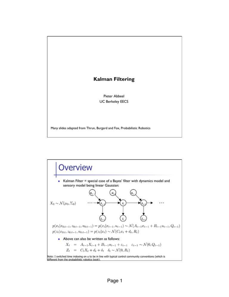
Kalman Filter = special case of a Bayes’ filter with dynamics model and
sensory model being linear Gaussian:
2
n
-1
Above can also be written as follows:
Note: I switched time indexing on u to be in line with typical control community conventions (which is
different from the probabilistic robotics book).
Page 1!
Time update
n
Assume we have current belief for
n
Then, after one time step passes:
:
Xt
Xt+1
Time Update: Finding the joint
n
Now we can choose to continue by either of
n
n
(i) mold it into a standard multivariate Gaussian format so
we can read of the joint distribution’s mean and covariance
(ii) observe this is a quadratic form in x_{t} and x_{t+1} in
the exponent; the exponent is the only place they appear;
hence we know this is a multivariate Gaussian. We directly
compute its mean and covariance. [usually simpler!]
Page 2!
Time Update: Finding the joint
n
We follow (ii) and find the means and covariance matrices in
[Exercise: Try to prove each of these
without referring to this slide!]
Time Update Recap
n
Assume we have
n
Then we have
n
Marginalizing the joint, we immediately get
Page 3!
Xt
Xt+1
Generality!
V
n
Assume we have
n
Then we have
n
Marginalizing the joint, we immediately get
Observation update
n
Assume we have:
n
Then:
n
W
Xt+1
Zt+1
And, by conditioning on
Gaussians) we readily get:
Page 4!
(see lecture slides on
Complete Kalman Filtering Algorithm
n
At time 0:
n
For t = 1, 2, …
n
Dynamics update:
n
Measurement update:
n
Often written as:
(Kalman gain)
“innovation”
Kalman Filter Summary
n
n
Highly efficient: Polynomial in measurement dimensionality k
and state dimensionality n:
O(k2.376 + n2)
Optimal for linear Gaussian systems!
10
Page 5!
Forthcoming Extensions
n
Nonlinear systems
n
n
Very large systems with sparsity structure
n
n
Extended Kalman Filter, Unscented Kalman Filter
Sparse Information Filter
Very large systems with low-rank structure
n
Ensemble Kalman Filter
n
Kalman filtering over SE(3)
n
How to estimate At, Bt, Ct, Qt, Rt from data (z0:T, u0:T)
n
n
EM algorithm
How to compute
n
(note the capital “T”)
Smoothing
Things to be aware of that we won’t cover
n
n
Square-root Kalman filter --- keeps track of square root of covariance matrices --equally fast, numerically more stable (bit more complicated conceptually)
If At = A, Qt = Q, Ct = C, Rt = R
n
If system is “observable” then covariances and Kalman gain will converge to
steady-state values for t -> 1
n
n
n
n
n
Can take advantage of this: pre-compute them, only track the mean, which is done by
multiplying Kalman gain with “innovation”
System is observable if and only if the following holds true: if there were zero
noise you could determine the initial state after a finite number of time steps
Observable if and only if: rank( [ C ; CA ; CA2 ; CA3 ; … ; CAn-1]) = n
Typically if a system is not observable you will want to add a sensor to make
it observable
Kalman filter can also be derived as the (recursively computed) least-squares
solutions to a (growing) set of linear equations
Page 6!