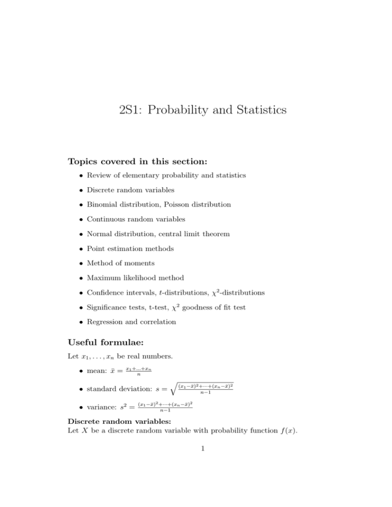
2S1: Probability and Statistics
Topics covered in this section:
• Review of elementary probability and statistics
• Discrete random variables
• Binomial distribution, Poisson distribution
• Continuous random variables
• Normal distribution, central limit theorem
• Point estimation methods
• Method of moments
• Maximum likelihood method
• Confidence intervals, t-distributions, χ2 -distributions
• Significance tests, t-test, χ2 goodness of fit test
• Regression and correlation
Useful formulae:
Let x1 , . . . , xn be real numbers.
• mean: x̄ =
x1 +...+xn
n
• standard deviation: s =
• variance: s2 =
q
(x1 −x̄)2 +···+(xn −x̄)2
n−1
(x1 −x̄)2 +···+(xn −x̄)2
n−1
Discrete random variables:
Let X be a discrete random variable with probability function f (x).
1
• probability: P (X = x) = f (x)
• cumulative distribution function: F (x) = P (X ≤ x)
P
• mean or expected value: µ = E(X) = j xj f (xj )
P
• variance: σ 2 = E[(X − µ)2 ] = j (xj − µ)2 f (xj )
If X is a discrete random variable with a binomial distribution then
n
• probability function: f (x) =
px (1 − p)n−x , x = 0, 1, . . . , n
x
where n = number of trials, p = probability of success in a trial.
• expected value: E(X) = np
• variance: var(X) = np(1 − p)
If X is a discrete random variable with a Poisson distribution then
• probability function: f (x) =
µx e−µ
,
x!
x = 0, 1, 2, . . ., where µ > 0
• expected value: E(X) = µ
• variance: var(X) = µ
Continuous random variables:
Let X be a continuous random variable with probability density function f (x).
Rb
• probability: P (a < X ≤ b) = a f (x) dx
• cumulative distribution function: F (x) = P (X ≤ x)
R∞
• mean or expected value: µ = E(X) = −∞ xf (x) dx
R∞
• variance: σ 2 = E[(X − µ)2 ] = −∞ (x − µ)2 f (x) dx
• standardized random variable: Z =
X−µ
σ
Let X be a continuous random variable with a normal distribution.
• probability density function: f (x) =
• expected value: E(X) = µ
• variance: var(X) = σ 2
2
√1
σ 2π
e−(x−µ)
2 /2σ 2
Point estimation:
Method of moments.
• kth population moment E(X k )
• kth sample moment
xkj
j=1 n
Pn
Maximum likelihood method to estimate unknown parameters θ1 , . . . , θr in a
probability distribution.
• Likelihood function: L(θ1 , . . . , θr ) = P (X = x1 ) . . . P (X = xn )
where x1 , . . . , xn is a random sample.
Confidence intervals:
For mean µ of a normal distribution with known variance σ 2 .
• [x̄ − z √σn , x̄ + z √σn ]
where n = sample size, Φ(z) =
1+γ
,
2
γ = confidence level.
• Use the normal distribution table to find z.
For mean µ of a normal distribution with unknown variance.
• [x̄ − z √sn , x̄ + z √sn ]
where n = sample size, s = sample standard deviation,
F (z) = 1+γ
, γ = confidence level.
2
• Use the t-distribution table with n − 1 degrees of freedom to find z.
For variance of a normal distribution.
2
2
• [ (n−1)s
, (n−1)s
]
z2
z1
where n = sample size, s2 = sample variance, F (z1 ) =
γ = confidence level.
1−γ
,
2
F (z2 ) =
1+γ
,
2
• Use the χ2 -distribution table with n − 1 degrees of freedom to find z1 and
z2 .
Significance tests:
Test to compare a value µ0 to the mean of a normal distribution with standard
deviation σ.
• If σ is known then use the random variable Z =
Use the normal distribution table.
3
x̄−µ
√0 .
σ/ n
√0 .
• If σ is unknown then use the random variable T = x̄−µ
s/ n
If the sample size is ≥ 25 then use the normal distribution table.
If the sample size is < 25 then use the t-distribution table with n−1 degrees
of freedom. (This is called a t-test).
Test to compare two sample means with the same standard deviation σ.
• If σ is known then use the random variable Z =
σ
x̄1 −x̄2
q
1
+ n1
n
1
2
where n1 , n2 are sample sizes and x̄1 , x̄2 are sample means.
Use the normal distribution table.
• If σ is unknown then use the random variable T = qx̄11−x̄2 1
s n +n
1
2
q
2
2
(n1 −1)s1 +(n2 −1)s2
where s =
n1 +n2 −2
2 2
and s1 , s2 are sample variances.
Use the t-distribution table with n1 + n2 − 2 degrees of freedom.
χ2 goodness of fit test.
• Partition the x-axis into subintervals I1 , . . . , Ik
P
(o −np )2
• Use the random variable χ2 = kj=1 j npj j
where oj = number of observed sample values in Ij
pj = probability that X takes a value in Ij , n = sample size.
• Use the χ2 -distribution table with k − 1 degrees of freedom.
4