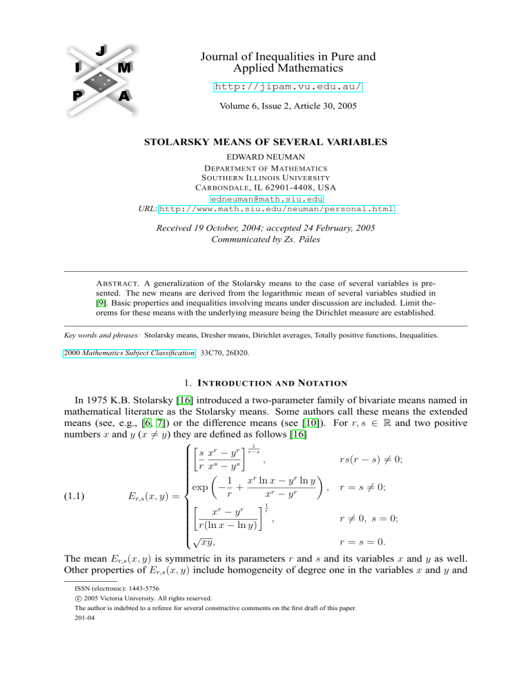
Journal of Inequalities in Pure and
Applied Mathematics
http://jipam.vu.edu.au/
Volume 6, Issue 2, Article 30, 2005
STOLARSKY MEANS OF SEVERAL VARIABLES
EDWARD NEUMAN
D EPARTMENT OF M ATHEMATICS
S OUTHERN I LLINOIS U NIVERSITY
C ARBONDALE , IL 62901-4408, USA
edneuman@math.siu.edu
URL: http://www.math.siu.edu/neuman/personal.html
Received 19 October, 2004; accepted 24 February, 2005
Communicated by Zs. Páles
A BSTRACT. A generalization of the Stolarsky means to the case of several variables is presented. The new means are derived from the logarithmic mean of several variables studied in
[9]. Basic properties and inequalities involving means under discussion are included. Limit theorems for these means with the underlying measure being the Dirichlet measure are established.
Key words and phrases: Stolarsky means, Dresher means, Dirichlet averages, Totally positive functions, Inequalities.
2000 Mathematics Subject Classification. 33C70, 26D20.
1. I NTRODUCTION
AND
N OTATION
In 1975 K.B. Stolarsky [16] introduced a two-parameter family of bivariate means named in
mathematical literature as the Stolarsky means. Some authors call these means the extended
means (see, e.g., [6, 7]) or the difference means (see [10]). For r, s ∈ R and two positive
numbers x and y (x 6= y) they are defined as follows [16]

1
 s xr − y r r−s



,
rs(r − s) 6= 0;

s − ys

r
x




r
r


exp − 1 + x ln x − y ln y , r = s 6= 0;
r
xr − y r
(1.1)
Er,s (x, y) =

r1



xr − y r


,
r 6= 0, s = 0;


r(ln
x
−
ln
y)



√

xy,
r = s = 0.
The mean Er,s (x, y) is symmetric in its parameters r and s and its variables x and y as well.
Other properties of Er,s (x, y) include homogeneity of degree one in the variables x and y and
ISSN (electronic): 1443-5756
c 2005 Victoria University. All rights reserved.
The author is indebted to a referee for several constructive comments on the first draft of this paper.
201-04
2
E DWARD N EUMAN
monotonicity in r and s. It is known that Er,s increases with an increase in either r or s (see
[6]). It is worth mentioning that the Stolarsky mean admits the following integral representation
([16])
Z s
1
(1.2)
ln Er,s (x, y) =
ln It dt
s−r r
(r 6= s), where It ≡ It (x, y) = Et,t (x, y) is the identric mean of order t. J. Pečarić and V. Šimić
[15] have pointed out that
Z
(1.3)
1
s
tx + (1 − t)y
Er,s (x, y) =
s
r−s
s
1
r−s
dt
0
(s(r − s) 6= 0). This representation shows that the Stolarsky means belong to a two-parameter
family of means studied earlier by M.D. Tobey [18]. A comparison theorem for the Stolarsky
means have been obtained by E.B. Leach and M.C. Sholander in [7] and independently by Zs.
Páles in [13]. Other results for the means (1.1) include inequalities, limit theorems and more
(see, e.g., [17, 4, 6, 10, 12]).
In the past several years researchers made an attempt to generalize Stolarsky means to several
variables (see [6, 18, 15, 8]). Further generalizations include so-called functional Stolarsky
means. For more details about the latter class of means the interested reader is referred to [14]
and [11].
To facilitate presentation let us introduce more notation. In what follows, the symbol En−1
will stand for the Euclidean simplex, which is defined by
En−1 = (u1 , . . . , un−1 ) : ui ≥ 0, 1 ≤ i ≤ n − 1, u1 + · · · + un−1 ≤ 1 .
Further, let X = (x1 , . . . , xn ) be an n-tuple of positive numbers and let Xmin = min(X),
Xmax = max(X). The following
Z
Z
n
Y
ui
exp(u · Z) du
(1.4)
L(X) = (n − 1)!
xi du = (n − 1)!
En−1 i=1
En−1
is the special case of the logarithmic mean of X which has been introduced in [9]. Here u =
(u1 , . . . , un−1 , 1 − u1 − · · · − un−1 ) where (u1 , . . . , un−1 ) ∈ En−1 , du = du1 . . . dun−1 , Z =
ln(X) = (ln x1 , . . . , ln xn ), and x · y = x1 y1 + · · · + xn yn is the dot product of two vectors x
and y. Recently J. Merikowski [8] has proposed the following generalization of the Stolarsky
mean Er,s to several variables
1
L(X r ) r−s
(1.5)
Er,s (X) =
L(X s )
(r 6= s), where X r = (xr1 , . . . , xrn ). In the paper cited above, the author did not prove that
Er,s (X) is the mean of X, i.e., that
(1.6)
Xmin ≤ Er,s (X) ≤ Xmax
holds true. If n = 2 and rs(r − s) 6= 0 or if r 6= 0 and s = 0, then (1.5) simplifies to (1.1) in
the stated cases.
This paper deals with a two-parameter family of multivariate means whose prototype is given
in (1.5). In order to define these means let us introduce more notation. By µ we will denote a
probability measure on En−1 . The logarithmic mean L(µ; X) with the underlying measure µ is
J. Inequal. Pure and Appl. Math., 6(2) Art. 30, 2005
http://jipam.vu.edu.au/
S TOLARSKY M EANS OF S EVERAL VARIABLES
3
defined in [9] as follows
Z
(1.7)
L(µ; X) =
n
Y
xui i µ(u) du
Z
exp(u · Z)µ(u) du.
=
En−1 i=1
En−1
We define
(1.8)

1
r−s
r

L(µ;
X
)


,

L(µ; X s )
Er,s (µ; X) =

d

r

exp
ln L(µ; X ) ,
dr
r 6= s
r = s.
Let us note that for µ(u) = (n − 1)!, the Lebesgue measure on En−1 , the first part of (1.8)
simplifies to (1.5).
In Section 2 we shall prove that Er,s (µ; X) is the mean value of X, i.e., it satisfies inequalities
(1.6). Some elementary properties of this mean are also derived. Section 3 deals with the limit
theorems for the new mean, with the probability measure being the Dirichlet measure. The
latter is denoted by µb , where b = (b1 , . . . , bn ) ∈ Rn+ , and is defined as [2]
n
1 Y bi −1
µb (u) =
u
,
B(b) i=1 i
(1.9)
where B(·) is the multivariate beta function, (u1 , . . . , un−1 ) ∈ En−1 , and un = 1 − u1 − · · · −
un−1 . In the Appendix we shall prove that under certain conditions imposed on the parameters
r−s
r and s, the function Er,s
(x, y) is strictly totally positive as a function of x and y.
2. E LEMENTARY P ROPERTIES OF Er,s (µ; X)
In order to prove that Er,s (µ; X) is a mean value we need the following version of the MeanValue Theorem for integrals.
Proposition 2.1. Let α := Xmin < Xmax =: β and let f, g ∈ C [α, β] with g(t) 6= 0 for all
t ∈ [α, β]. Then there exists ξ ∈ (α, β) such that
R
f (u · X)µ(u) du
f (ξ)
REn−1
(2.1)
=
.
g(ξ)
g(u · X)µ(u) du
En−1
Proof. Let the numbers γ and δ and the function φ be defined in the following way
Z
Z
γ=
g(u · X)µ(u) du,
δ=
f (u · X)µ(u) du,
En−1
En−1
φ(t) = γf (t) − δg(t).
Letting t = u · X and, next, integrating both sides against the measure µ, we obtain
Z
φ(u · X)µ(u) du = 0.
En−1
On the other hand, application of the Mean-Value Theorem to the last integral gives
Z
φ(c · X)
µ(u) du = 0,
En−1
J. Inequal. Pure and Appl. Math., 6(2) Art. 30, 2005
http://jipam.vu.edu.au/
4
E DWARD N EUMAN
where c = (c1 , . . . , cn−1 , cn ) with (c1 , . . . , cn−1 ) ∈ En−1 and cn = 1 − c1 − · · · − cn−1 . Letting
ξ = c · X and taking into account that
Z
µ(u) du = 1
En−1
we obtain φ(ξ) = 0. This in conjunction with the definition of φ gives the desired result (2.1).
The proof is complete.
The author is indebted to Professor Zsolt Páles for a useful suggestion regarding the proof of
Proposition 2.1.
(p)
For later use let us introduce the symbol Er,s (µ; X) (p 6= 0), where
1
(p)
(2.2)
Er,s
(µ; X) = Er,s (µ; X p ) p .
We are in a position to prove the following.
Theorem 2.2. Let X ∈ Rn+ and let r, s ∈ R. Then
(i) Xmin ≤ Er,s (µ; X) ≤ Xmax ,
(ii) Er,s (µ; λX) = λEr,s (µ; X), λ > 0, (λX := (λx1 , . . . , λxn )),
(iii) Er,s (µ; X) increases with an increase in either r and s,
1 Rr
(iv) ln Er,s (µ; X) =
ln Et,t (µ; X) dt , r 6= s,
r−s s
(p)
(v) Er,s (µ; X) = Epr,ps (µ; X),
(vi) Er,s (µ; X)E−r,−s (µ; X −1 ) = 1, (X −1 := (1/x1 , . . . , 1/xn )),
s−r
p−r
s−p
(vii) Er,s
(µ; X) = Er,p
(µ; X)Ep,s
(µ; X).
Proof of (i). Assume first that r 6= s. Making use of (1.8) and (1.7) we obtain
1
"R
# r−s
exp
r(u
·
Z)
µ(u)
du
E
Er,s (µ; X) = R n−1
.
exp
s(u
·
Z)
µ(u)
du
En−1
Application of (2.1) with f (t) = exp(rt) and g(t) = exp(st) gives
"
# 1
exp r(c · Z) r−s
Er,s (µ; X) =
= exp(c · Z),
exp s(c · Z)
where c = (c1 , . . . , cn−1 , cn ) with (c1 , . . . , cn−1 ) ∈ En−1 and cn = 1 − c1 − · · · − cn−1 . Since
c · Z = c1 ln x1 + · · · + cn ln xn , ln Xmin ≤ c · Z ≤ ln Xmax . This in turn implies that
Xmin ≤ exp(c · Z) ≤ Xmax . This completes the proof of (i) when r 6= s. Assume now that
r = s. It follows from (1.8) and (1.7) that
"R
#
(u
·
Z)
exp
r(u
·
Z)
µ(u)
du
En−1
R
ln Er,r (µ; X) =
.
exp
r(u
·
Z)
µ(u)
du
En−1
Application of (2.1) to the right side with f (t) = t exp(rt) and g(t) = exp(rt) gives
"
#
(c · Z) exp r(c · Z)
ln Er,r (µ; X) =
= c · Z.
exp r(c · Z)
Since ln Xmin ≤ c · Z ≤ ln Xmax , the assertion follows. This completes the proof of (i).
Proof of (ii). The following result
(2.3)
L µ; (λx)r = λr L(µ; X r )
J. Inequal. Pure and Appl. Math., 6(2) Art. 30, 2005
http://jipam.vu.edu.au/
S TOLARSKY M EANS OF S EVERAL VARIABLES
5
(λ > 0) is established in [9, (2.6)]. Assume that r 6= s. Using (1.8) and (2.3) we obtain
r
1
λ L(µ; X r ) r−s
Er,s (µ; λx) = s
= λEr,s (µ; X).
λ L(µ; X s )
Consider now the case when r = s 6= 0. Making use of (1.8) and (2.3) we obtain
d
r
ln L µ; (λX)
Er,r (µ; λX) = exp
dr
d
r
r
= exp
ln λ L(µ; X )
dr
d
r
= exp
r ln λ + ln L(µ; X ) = λEr,r (µ; X).
dr
When r = s = 0, an easy computation shows that
(2.4)
n
Y
E0,0 (µ; X) =
i
xw
i ≡ G(w; X),
i=1
where
Z
wi =
(2.5)
ui µ(u) du
En−1
(1 ≤ i ≤ n) are called the natural weights or partial moments of the measure µ and w =
(w1 , . . . , wn ). Since w1 + · · · + wn = 1, E0,0 (µ; λX) = λE0,0 (µ; X). The proof of (ii) is
complete.
Proof of (iii). In order to establish the asserted property, let us note that the function r →
exp(rt) is logarithmically convex (log-convex) in r. This in conjunction with Theorem B.6 in
[2], implies that a function r → L(µ; X r ) is also log-convex in r. It follows from (1.8) that
ln Er,s (µ; X) =
ln L(µ; X r ) − ln L(µ; X s )
.
r−s
The right side is the divided difference of order one at r and s. Convexity of ln L(µ; X r ) in
r implies that the divided difference increases with an increase in either r and s. This in turn
implies that ln Er,s (µ; X) has the same property. Hence the monotonicity property of the mean
Er,s in its parameters follows. Now let r = s. Then (1.8) yields
ln Er,r (µ; X) =
d
ln L(µ; X r ) .
dr
Since ln L(µ; X r ) is convex in r, its derivative with respect to r increases with an increase in r.
This completes the proof of (iii).
Proof of (iv). Let r 6= s. It follows from (1.8) that
Z r
Z r
1
1
d
ln Et,t (µ; X) dt =
ln L(µ; X t ) dt
r−s s
r − s s dt
1 =
ln L(µ; X r ) − ln L(µ; X s )
r−s
= ln Er,s (µ; X).
J. Inequal. Pure and Appl. Math., 6(2) Art. 30, 2005
http://jipam.vu.edu.au/
6
E DWARD N EUMAN
Proof of (v). Let r 6= s. Using (2.2) and (1.8) we obtain
1
1
L(X pr ) p(r−s)
p p
(p)
= Epr,ps (µ; X).
Er,s (µ; X) = Er,s (µ; X ) =
L(X ps )
Assume now that r = s 6= 0. Making use of (2.2), (1.8) and (1.7) we have
1 d
(p)
pr
Er,r (µ; X) = exp
ln L(µ; X )
p dr
Z
1
= exp
(u · Z) exp pr(u · Z) µ(u) du
L(µ; X pr ) En−1
= Epr,pr (µ; X).
The case when r = s = 0 is trivial because E0,0 (µ; X) is the weighted geometric mean of X.
Proof of (vi). Here we use (v) with p = −1 to obtain Er,s (µ; X −1 )−1 = E−r,−s (µ; X). Letting
X := X −1 we obtain the desired result.
Proof of (vii). There is nothing to prove when either p = r or p = s or r = s. In other cases we
use (1.8) to obtain the asserted result. This completes the proof.
In the next theorem we give some inequalities involving the means under discussion.
Theorem 2.3. Let r, s ∈ R. Then the following inequalities
(2.6)
Er,r (µ; X) ≤ Er,s (µ; X) ≤ Es,s (µ; X)
are valid provided r ≤ s. If s > 0, then
(2.7)
Er−s,0 (µ; X) ≤ Er,s (µ; X).
Inequality (2.7) is reversed if s < 0 and it becomes an equality if s = 0. Assume that r, s > 0
and let p ≤ q. Then
(p)
(q)
Er,s
(µ; X) ≤ Er,s
(µ; X)
(2.8)
with the inequality reversed if r, s < 0.
Proof. Inequalities (2.6) and (2.7) follow immediately from Part (iii) of Theorem 2.2. For the
proof of (2.8), let r, s > 0 and let p ≤ q. Then pr ≤ qr and ps ≤ qs. Applying Parts (v) and
(iii) of Theorem 2.2, we obtain
(p)
(q)
Er,s
(µ; X) = Epr,ps (µ; X) ≤ Eqr,qs (µ; X) = Er,s
(µ; X).
When r, s < 0, the proof of (2.8) goes along the lines introduced above, hence it is omitted.
The proof is complete.
3. T HE M EAN Er,s (b; X)
An important probability measure on En−1 is the Dirichlet measure µb (u), b ∈ Rn+ (see (1.9)).
Its role in the theory of special functions is well documented in Carlson’s monograph [2]. When
µ = µb , the mean under discussion will be denoted by Er,s (b; X). The natural weights wi (see
(2.5)) of µb are given explicitly by
(3.1)
J. Inequal. Pure and Appl. Math., 6(2) Art. 30, 2005
wi = bi /c
http://jipam.vu.edu.au/
S TOLARSKY M EANS OF S EVERAL VARIABLES
7
(1 ≤ i ≤ n), where c = b1 +· · ·+bn (see [2, (5.6-2)]). For later use we define w = (w1 , . . . , wn ).
Recall that the weighted Dresher mean Dr,s (p; X) of order (r, s) ∈ R2 of X ∈ Rn+ with weights
p = (p1 , . . . , pn ) ∈ Rn+ is defined as
P
1
n
r r−s

p
i xi

i=1

Pn
,
r 6= s

s


i=1 pi xi
(3.2)
Dr,s (p; X) =

Pn


pi xri ln xi

i=1

Pn
exp
, r=s
r
i=1 pi xi
(see, e.g., [1, Sec. 24]).
In this section we present two limit theorems for the mean Er,s with the underlying measure being the Dirichlet measure. In order to facilitate presentation we need a concept of the
Dirichlet average of a function. Following [2, Def. 5.2-1] let Ω be a convex set in C and let
Y = (y1 , . . . , yn ) ∈ Ωn , n ≥ 2. Further, let f be a measurable function on Ω. Define
Z
(3.3)
F (b; Y ) =
f (u · Y )µb (u) du.
En−1
Then F is called the Dirichlet average of f with variables Y = (y1 , . . . , yn ) and parameters
b = (b1 , . . . , bn ). We need the following result [2, Ex. 6.3-4]. Let Ω be an open circular disk in
C, and let f be holomorphic on Ω. Let Y ∈ Ωn , c ∈ C, c 6= 0, −1, . . ., and w1 + · · · + wn = 1.
Then
n
X
(3.4)
lim F (cw; Y ) =
wi f (yi ),
c→0
i=1
where cw = (cw1 , . . . , cwn ).
We are in a position to prove the following.
Theorem 3.1. Let w1 > 0, . . . , wn > 0 with w1 + · · · + wn = 1. If r, s ∈ R and X ∈ Rn+ , then
lim Er,s (cw; X) = Dr,s (w; X).
c→0+
Proof. We use (1.7) and (3.3) to obtain L(cw; X) = F (cw; Z), where Z = ln X = (ln x1 , . . . , ln xn ).
Making use of (3.4) with f (t) = exp(t) and Y = ln X we obtain
lim L(cw; X) =
c→0+
n
X
wi xi .
i=1
Hence
lim+ L(cw; X r ) =
(3.5)
c→0
n
X
wi xri .
i=1
Assume that r 6= s. Application of (3.5) to (1.8) gives
1
Pn
1
wi xri r−s
L(cw; X r ) r−s
i=1
lim Er,s (cw; X) = lim+
= Pn
= Dr,s (w; X).
s
c→0+
c→0
L(cw; X s )
i=1 wi xi
Let r = s. Application of (3.4) with f (t) = t exp(rt) gives
lim F (cw; Z) =
c→0+
J. Inequal. Pure and Appl. Math., 6(2) Art. 30, 2005
n
X
i=1
wi zi exp(rzi ) =
n
X
wi (ln xi )xri .
i=1
http://jipam.vu.edu.au/
8
E DWARD N EUMAN
This in conjunction with (3.5) and (1.8) gives
Pn
wi xri ln xi
F (cw; Z)
i=1
Pn
lim Er,r (cw; X) = lim+ exp
= Dr,r (w; X).
= exp
r
c→0+
c→0
L(cw; X r )
i=1 wi xi
This completes the proof.
Theorem 3.2. Under the assumptions of Theorem 3.1 one has
lim Er,s (cw; X) = G(w; X).
(3.6)
c→∞
Proof. The following limit (see [9, (4.10)])
lim L(cw; X) = G(w; X)
(3.7)
c→∞
will be used in the sequel. We shall establish first (3.6) when r 6= s. It follows from (1.8) and
(3.7) that
1
1
L(cw; X r ) r−s r−s r−s
=
G(w;
X)
= G(w; X).
lim Er,s (cw; X) = lim
c→∞
c→∞ L(cw; X s )
Assume that r = s. We shall prove first that
(3.8)
lim F (cw; Z) = ln G(w; X) G(w; X)r ,
c→∞
where F is the Dirichlet average of f (t) = t exp(rt). Averaging both sides of
∞
X
rm m+1
f (t) =
t
m!
m=0
we obtain
F (cw; Z) =
(3.9)
∞
X
rm
Rm+1 (cw; Z),
m!
m=0
where Rm+1 stands for the Dirichlet average of the power function tm+1 . We will show that the
series in (3.9) converges uniformly in 0 < c < ∞. This in turn implies further that as c → ∞,
we can proceed to the limit term by term. Making use of [2, 6.2-24)] we obtain
|Rm+1 (cw; Z)| ≤ |Z|m+1 ,
m ∈ N,
where |Z| = max | ln xi | : 1 ≤ i ≤ n . By the Weierstrass M test the series in (3.9) converges
uniformly in the stated domain. Taking limits on both sides of (3.9) we obtain with the aid of
(3.4)
∞
X
rm
lim F (cw; Z) =
lim Rm+1 (cw; Z)
c→∞
m! c→∞
m=0
!m+1
∞
n
X
rm X
=
wi zi
m! i=1
m=0
∞
X
m
rm = ln G(w; X)
ln G(w; X)
m!
m=0
∞
X
m
1 = ln G(w; X)
ln G(w; X)r
m!
m=0
= ln G(w; X) G(w; X)r .
J. Inequal. Pure and Appl. Math., 6(2) Art. 30, 2005
http://jipam.vu.edu.au/
S TOLARSKY M EANS OF S EVERAL VARIABLES
9
This completes the proof of (3.8). To complete the proof of (3.6) we use (1.8), (3.7), and (3.8)
to obtain
ln G(w; X) G(w; X)r
F (cw; Z)
lim ln Er,r (µ; X) = lim
=
= ln G(w; X).
c→∞
c→∞ L(cw; X r )
G(w; X)r
Hence the assertion follows.
A PPENDIX A. T OTAL P OSITIVITY
OF
r−s
Er,s
(x, y)
A real-valued function h(x, y) of two real variables is said to be strictly totally positive on
its domain if every n × n determinant with elements h(xi , yj ), where x1 < x2 < · · · < xn and
y1 < y2 < · · · < yn is strictly positive for every n = 1, 2, . . . (see [5]).
r−s
The goal of this section is to prove that the function Er,s
(x, y) is strictly totally positive as a
function of x and y provided the parameters r and s satisfy a certain condition. For later use we
recall the definition of the R-hypergeometric function R−α (β, β 0 ; x, y) of two variables x, y > 0
with parameters β, β 0 > 0
Z
−α
Γ(β + β 0 ) 1 β−1
0
0
(A1)
R−α (β, β ; x, y) =
u (1 − u)β −1 ux + (1 − u)y
du
0
Γ(β)Γ(β ) 0
(see [2, (5.9-1)]).
r−s
Proposition A.1. Let x, y > 0 and let r, s ∈ R. If |r| < |s|, then Er,s
(x, y) is strictly totally
positive on R2+ .
Proof. Using (1.3) and (A1) we have
(A2)
r−s
Er,s
(x, y) = R r−s (1, 1; xs , y s )
s
(s(r − s) 6= 0). B. Carlson and J. Gustafson [3] have proven that R−α (β, β 0 ; x, y) is strictly
totally positive in x and y provided β, β 0 > 0 and 0 < α < β + β 0 . Letting α = 1 − r/s,
β = β 0 = 1, x := xs , y := y s , and next, using (A2) we obtain the desired result.
Corollary A.2. Let 0 < x1 < x2 , 0 < y1 < y2 and let the real numbers r and s satisfy the
inequality |r| < |s|. If s > 0, then
(A3)
Er,s (x1 , y1 )Er,s (x2 , y2 ) < Er,s (x1 , y2 )Er,s (x2 , y1 ).
Inequality (A3) is reversed if s < 0.
r−s
Proof. Let aij = Er,s
(xi , yj ) (i, j = 1, 2). It follows from Proposition A.1 that det [aij ] > 0
provided |r| < |s|. This in turn implies
r−s r−s
Er,s (x1 , y1 )Er,s (x2 , y2 )
> Er,s (x1 , y2 )Er,s (x2 , y1 )
.
Assume that s > 0. Then the inequality |r| < s implies r − s < 0. Hence (A3) follows when
s > 0. The case when s < 0 is treated in a similar way.
R EFERENCES
[1] E.F. BECKENBACH AND R. BELLMAN, Inequalities, Springer-Verlag, Berlin, 1961.
[2] B.C. CARLSON, Special Functions of Applied Mathematics, Academic Press, New York, 1977.
[3] B.C. CARLSON AND J.L. GUSTAFSON, Total positivity of mean values and hypergeometric functions, SIAM J. Math. Anal., 14(2) (1983), 389–395.
[4] P. CZINDER AND ZS . PÁLES An extension of the Hermite-Hadamard inequality and an application for Gini and Stolarsky means, J. Ineq. Pure Appl. Math., 5(2) (2004), Art. 42. [ONLINE:
http://jipam.vu.edu.au/article.php?sid=399].
J. Inequal. Pure and Appl. Math., 6(2) Art. 30, 2005
http://jipam.vu.edu.au/
10
E DWARD N EUMAN
[5] S. KARLIN, Total Positivity, Stanford Univ. Press, Stanford, CA, 1968.
[6] E.B. LEACH AND M.C. SHOLANDER, Extended mean values, Amer. Math. Monthly, 85(2)
(1978), 84–90.
[7] E.B. LEACH AND M.C. SHOLANDER, Multi-variable extended mean values, J. Math. Anal.
Appl., 104 (1984), 390–407.
[8] J.K. MERIKOWSKI, Extending means of two variables to several variables, J. Ineq. Pure Appl.
Math., 5(3) (2004), Art. 65. [ONLINE: http://jipam.vu.edu.au/article.php?sid=
411].
[9] E. NEUMAN, The weighted logarithmic mean, J. Math. Anal. Appl., 188 (1994), 885–900.
[10] E. NEUMAN AND ZS . PÁLES, On comparison of Stolarsky and Gini means, J. Math. Anal.
Appl., 278 (2003), 274–284.
[11] E. NEUMAN, C.E.M. PEARCE, J. PEČARIĆ AND V. ŠIMIĆ, The generalized Hadamard inequality, g-convexity and functional Stolarsky means, Bull. Austral. Math. Soc., 68 (2003), 303–316.
[12] E. NEUMAN AND J. SÁNDOR, Inequalities involving Stolarsky and Gini means, Math. Pannonica, 14(1) (2003), 29–44.
[13] ZS. PÁLES, Inequalities for differences of powers, J. Math. Anal. Appl., 131 (1988), 271–281.
[14] C.E.M. PEARCE, J. PEČARIĆ
Appl., 2 (1999), 479–489.
AND
V. ŠIMIĆ, Functional Stolarsky means, Math. Inequal.
[15] J. PEČARIĆ AND V. ŠIMIĆ, The Stolarsky-Tobey mean in n variables, Math. Inequal. Appl., 2
(1999), 325–341.
[16] K.B. STOLARSKY, Generalizations of the logarithmic mean, Math. Mag., 48(2) (1975), 87–92.
[17] K.B. STOLARSKY, The power and generalized logarithmic means, Amer. Math. Monthly, 87(7)
(1980), 545–548.
[18] M.D. TOBEY, A two-parameter homogeneous mean value, Proc. Amer. Math. Soc., 18 (1967),
9–14.
J. Inequal. Pure and Appl. Math., 6(2) Art. 30, 2005
http://jipam.vu.edu.au/