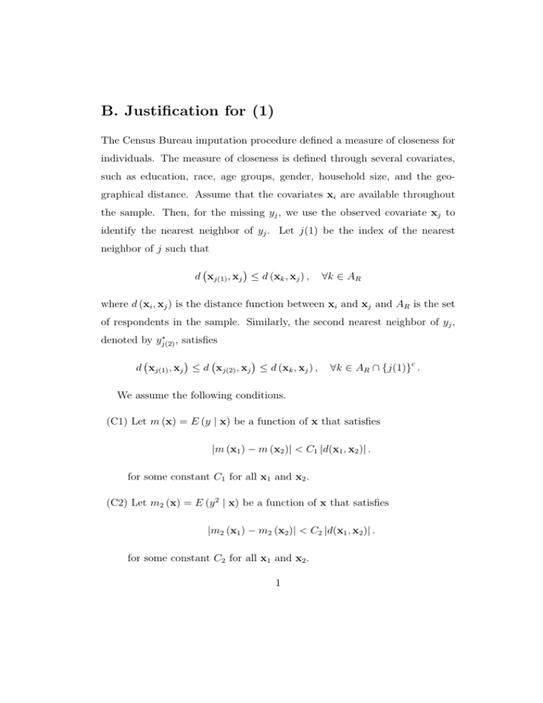
B. Justification for (1)
The Census Bureau imputation procedure defined a measure of closeness for
individuals. The measure of closeness is defined through several covariates,
such as education, race, age groups, gender, household size, and the geographical distance. Assume that the covariates xi are available throughout
the sample. Then, for the missing yj , we use the observed covariate xj to
identify the nearest neighbor of yj . Let j(1) be the index of the nearest
neighbor of j such that
(
)
d xj(1) , xj ≤ d (xk , xj ) ,
∀k ∈ AR
where d (xi , xj ) is the distance function between xi and xj and AR is the set
of respondents in the sample. Similarly, the second nearest neighbor of yj ,
∗
denoted by yj(2)
, satisfies
(
)
(
)
d xj(1) , xj ≤ d xj(2) , xj ≤ d (xk , xj ) ,
∀k ∈ AR ∩ {j(1)}c .
We assume the following conditions.
(C1) Let m (x) = E (y | x) be a function of x that satisfies
|m (x1 ) − m (x2 )| < C1 |d(x1 , x2 )| .
for some constant C1 for all x1 and x2 .
(C2) Let m2 (x) = E (y 2 | x) be a function of x that satisfies
|m2 (x1 ) − m2 (x2 )| < C2 |d(x1 , x2 )| .
for some constant C2 for all x1 and x2 .
1
(C3) For each i ∈ U , the cumulative distribution of d(x) = d(xi , x), denoted
by F (d), satisfies
lim F (d)/d > 0,
d→0
where it is understood that F (0) > 0 satisfies the condition.
(
)
∑
(C4) The sampling design is such that V N −1 i∈A πi−1 zi = O(n−1 ) for
any z with bounded fourth moments and πi > πL > 0 for all i
for some πL . The response probability satisfies P r (δi = 1 | xi , yi ) =
P r (δi = 1 | xi ) > 0 for all i.
Under the above regularity conditions, we can prove the following theorem.
Theorem 1 Let (xi , yi ) be the IID sample from a distribution with second
∗
∗
moments. Assume (C1)-(C4) holds. Let yj(1)
and yj(2)
be the first nearest
neighbor and the second nearest neighbor of yj , respectively. Then, we have
( ∗
)
(
)
| x∗j(1) = Op n−1+α
max E (yj | xj ) − E yj(1)
(B.1)
( ∗
)
(
)
max E (yj | xj ) − E yj(2)
| x∗j(2) = Op n−1+α
(B.2)
j
and
j
for any α > 0.
Proof. Define dij = d (xi , xj ) for i ̸= j and let dj(1) be the smallest value of
(
)
dij among i ∈ A ∩ {j}c . By definition, dj(1) = d xj , xj(1) . Similarly, we can
2
(
)
define dj(2) = d xj , xj(2) . Note that, for an = n1−α ,
(
)
P r max an dj(1) > M
=
j
n
∑
(
)
P r dj(1) > M/an
j=1
= n [1 − F (M/an )]n
= n exp [an nα log {1 − F (M/an )}]
≤ n exp [−an nα F (M/an )] ,
since log(1 − x) ≤ −x for x ∈ [0, 1). Thus, writing t = M/an , we have
(
)
P r max an dj(1) > M
≤ n exp [−M nα F (t) /t]
j
which goes to zero as n → ∞, since, by (C3), F (t) /t is bounded below by
some constant greater than zero. Thus, we have maxj an dj(1) = Op (1) and,
by (C1), we have (B.1).
To prove (B.2), we use
(
)
P r max an dj(2) > M
j
=
n
∑
(
)
P r dj(2) > M/an
j=1
[
]
= n {1 − F (M/an )}n + n {1 − F (M/an )}n−1 F (M/an )
= n {1 − F (M/an )}n−1 {1 + (n − 1)F (M/an )}
= n exp [(an nα − 1) log {1 − F (M/an )}] {1 + (n − 1)F (M/an )}
≤ n exp(1) exp [−an nα F (M/an )] {1 + nF (M/an )}
= Kn2 exp [−M nα F (t) /t] ,
for some K where t = M/an .
Thus, for any ϵ > 0, we have
(
)
P r maxj an dj(2) > M ≤ ϵ for sufficiently large n. Therefore, we have
maxj an dj(2) = Op (1) and, by (C1), (A2) is proved.
3
Similarly, it can be shown that, by assumption (C2),
(
)
( 2
)
(
)
max E yj2 | xj − E yj(1)
| xj(1) = Op n−1+α
j
and
(
)
( 2
)
(
)
| xj(1) = Op n−1+α .
max E yj2 | xj − E yj(2)
j
Thus, ignoring the smaller order terms and assuming the yj are independent
(
)
yi ∼ µj , σj2
i ∈ {j, j(1), j(2)} ,
and (1) is an adequate approximation for large n.
4
(B.3)