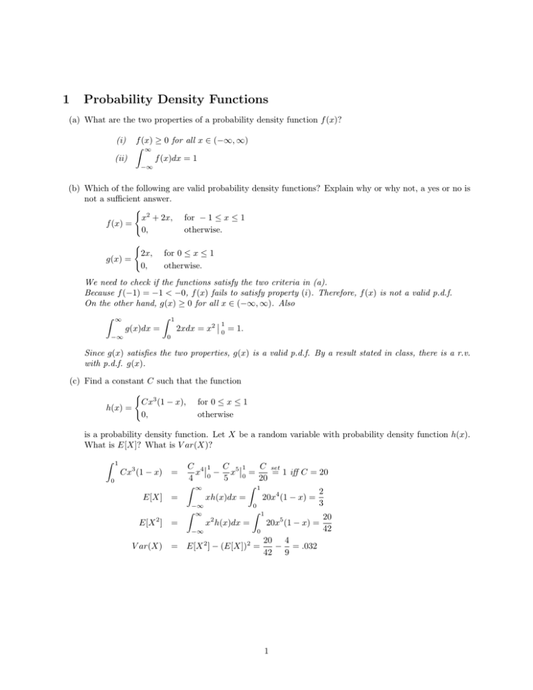
1
Probability Density Functions
(a) What are the two properties of a probability density function f (x)?
f (x) ≥ 0 for all x ∈ (−∞, ∞)
Z ∞
(ii)
f (x)dx = 1
(i)
−∞
(b) Which of the following are valid probability density functions? Explain why or why not, a yes or no is
not a sufficient answer.
(
x2 + 2x, for − 1 ≤ x ≤ 1
f (x) =
0,
otherwise.
(
2x,
g(x) =
0,
for 0 ≤ x ≤ 1
otherwise.
We need to check if the functions satisfy the two criteria in (a).
Because f (−1) = −1 < −0, f (x) fails to satisfy property (i). Therefore, f (x) is not a valid p.d.f.
On the other hand, g(x) ≥ 0 for all x ∈ (−∞, ∞). Also
Z
∞
Z
g(x)dx =
−∞
0
1
1
2xdx = x2 0 = 1.
Since g(x) satisfies the two properties, g(x) is a valid p.d.f. By a result stated in class, there is a r.v.
with p.d.f. g(x).
(c) Find a constant C such that the function
(
Cx3 (1 − x), for 0 ≤ x ≤ 1
h(x) =
0,
otherwise
is a probability density function. Let X be a random variable with probability density function h(x).
What is E[X]? What is V ar(X)?
Z
1
Cx3 (1 − x)
=
E[X]
=
E[X 2 ]
=
V ar(X)
=
0
C set
C 4 1 C 5 1
x 0− x 0=
= 1 iff C = 20
4
5
20
Z ∞
Z 1
2
xh(x)dx =
20x4 (1 − x) =
3
−∞
0
Z ∞
Z 1
20
x2 h(x)dx =
20x5 (1 − x) =
42
−∞
0
20
4
E[X 2 ] − (E[X])2 =
− = .032
42 9
1
2
Cumulative Distribution Functions
(a) State the three properties of a cumulative distribution function F (x).
(i)
F(x) is non-decreasing
(ii)
F(x) is right-continuous
(iii)
lim F (x) = 0, and lim F (x) = 1
x→−∞
x→∞
(b) Find expected value and variance of the random variable X with cumulative distribution function
0
for t < 0
FX (t) =
1 − e−3t for t ≥ 0
Also, find P (X ≤ 5) and P (X > 7). First, differentiate FX (t) with respect to t (at points where FX (t)
is differentiable) to find the p.d.f. fX (t) corresponding to FX (t):
(
dFX (t)
= 3e−3t , for 0 < x
dt
fX (t) =
0,
otherwise
Now, use the definition of the expected value of a continuous random variable to compute E[X].
Z ∞
Z ∞
E[X] =
xfX (x)dx =
3xe−3x = 1/3.
−∞
0
R
Integration by parts ( udv = uv − vdu), with dv = e−3x dx and u = 3x can be used to compute the
integral above. If you’re rusty on integration by parts, check out your old calculus notes, or (better
yet), come ask me!
To compute V ar(X), we can use the formula V ar(X) = E[X 2 ] − (E[X])2 . Another application of
integration by parts (again, if this integration by parts business is confusing you, come ask me) gives
Z ∞
2
E[X ] =
3x2 e−3x dx = 2/9
R
0
V ar(X)
=
2/9 − 1/9 = 1/9
Finally,
P (X ≤ .5)
=
FX (.5) = 1 − e−1.5 = 0.78
P (X > 1/3)
=
1 − FX (1/3) = e−1 = 0.37
(c) Find the c.d.f of the random variable X with p.d.f. h(x) given in part (c) of Problem 2 above. What
is P (X ≤ .5)?
The c.d.f. of X is
Z
H(x) =
0
x


0
h(t)dt = 5x4 − 4x5


1
for x < 0,
for 0 ≤ x < 1,
for x ≥ 1
Using the c.d.f,
P (X ≤ .5) = H(.5) = 5/16 − 4/32 = 0.1875.
2
3
Uniform Distribution
A 5 meter string is cut at a random point. (The cut point is chosen uniformly on the interval from 0 to
5). What is the probability that the longer piece is more than twice the length of the shorter piece? Let
W be the cut point. Then W ∼ U(0, 5). The longer piece is more than twice the length of the shorter piece
provided
5
10
or W < .
W > 2(5 − W ) or 2W < (5 − W ) ↔ W >
3
3
Since
Z 53
5
1
1
P (W < ) =
dx = , and
3
3
0 5
Z 1
1
1
10
) =
dx = ,
P (W >
10 5
3
3
3
P (W <
4
5
10
5
10
2
or W >
) = P (W < ) + P (W >
)= .
3
3
3
3
3
Robodogs
Imagine you and your friend have built your own Robodogs. Now, you want to battle against each other
(the Robodogs are going to bark at each other until the battery of one of them gives up). Using the same
kind of batteries you know that your Robodog lasts on average for five hours, while your friend’s Robodog
lasts for four hours.
Let X be the time until your Robodog’s battery stops working and Y be the time until your friend’s Robodog
stops barking.
Assume further, that X and Y are exponentially distributed variables, i.e. X ∼ Expλ , Y ∼ Expµ .
(a) Find µ and λ.
the expected value of an exponential distribution is 1/λ. As the average battery life times are reported
to be 5h and 4h respectively, λ = 0.2 and µ = 0.25
(b) Let Z be the time until the contest is over, i.e. until one of the dogs stops barking. Z can then be
written as Z = min (X, Y ).
Find the distribution of Z, i.e. compute P (Z ≤ z).
Hint: min (X, Y ) ≤ z ≡ (X ≤ z) ∪ (Y ≤ z); you can also assume that X and Y are independent
variables.
This question involves a little bit of math.
P (Z ≤ z)
hint
= P (min (X, Y ) ≤ z) = P ((X ≤ z) ∪ (Y ≤ z)) =
= P (X ≤ z) + P (Y ≤ z) − P ((X ≤ z) ∩ (Y ≤ z)) =
X,Y ind.
=
1 − eλz + 1 − e−µz − P ((X ≤ z) ∩ (Y ≤ z))
=
1 − eλz + 1 − e−µz − P (X ≤ z) · P (Y ≤ z) =
=
1 − eλz + 1 − e−µz − (1 − eλz ) · (1 − e−µz ) =
=
1 − eλz + 1 − e−µz − (1 − eλz − 1 − e−µz + e−λz−µz =
=
1 − e−(λ+µ)z ,
i.e. Z has an exponential distribution again! Z ∼ Exp0.2+0.25 !
3
=
(c) Do you recognize the distribution of Z? State expected value and variance. Interpret the expected
value. E[Z] = 1/0.45 = 2.22, V ar[Z] = 1/0.452 = 4.94
on average the contest is over in 2.22 hours.
4