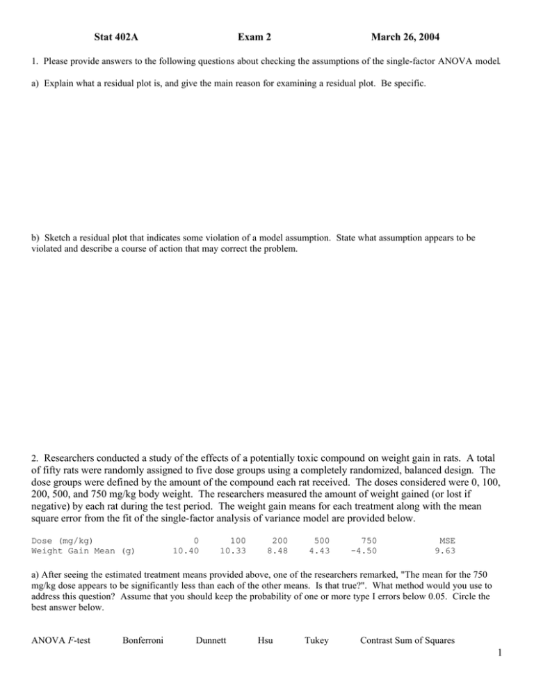
Stat 402A
Exam 2
March 26, 2004
1. Please provide answers to the following questions about checking the assumptions of the single-factor ANOVA model.
a) Explain what a residual plot is, and give the main reason for examining a residual plot. Be specific.
b) Sketch a residual plot that indicates some violation of a model assumption. State what assumption appears to be
violated and describe a course of action that may correct the problem.
2. Researchers conducted a study of the effects of a potentially toxic compound on weight gain in rats. A total
of fifty rats were randomly assigned to five dose groups using a completely randomized, balanced design. The
dose groups were defined by the amount of the compound each rat received. The doses considered were 0, 100,
200, 500, and 750 mg/kg body weight. The researchers measured the amount of weight gained (or lost if
negative) by each rat during the test period. The weight gain means for each treatment along with the mean
square error from the fit of the single-factor analysis of variance model are provided below.
Dose (mg/kg)
Weight Gain Mean (g)
0
10.40
100
10.33
200
8.48
500
4.43
750
-4.50
MSE
9.63
a) After seeing the estimated treatment means provided above, one of the researchers remarked, "The mean for the 750
mg/kg dose appears to be significantly less than each of the other means. Is that true?". What method would you use to
address this question? Assume that you should keep the probability of one or more type I errors below 0.05. Circle the
best answer below.
ANOVA F-test
Bonferroni
Dunnett
Hsu
Tukey
Contrast Sum of Squares
1
2. (continued)
b) Prior to collecting the data, one of the researchers said that there would be evidence of toxicity if any one of the
nonzero doses had a mean weight gain that was significantly less than the mean for the 0 dose treatment. If the
researchers want to keep the probability of making one or more type I errors below 0.05, what method would be best for
testing for toxicity using this criterion? Circle the best answer below.
ANOVA F-test
Bonferroni
Dunnett
Hsu
Tukey
Linear Combination of Means
c) Another researcher said that there would be evidence of toxicity if weight gain tended to decrease as the dose
increased. She decided to use Tukey's method for making all pairwise comparisons of treatment means. She obtained the
table below by issuing the SAS command lsmeans dose / adjust=Tukey pdiff;.
i/j
0
100
200
500
750
0
1.0000
0.6412
0.0008
<.0001
100
200
500
750
1.0000
0.6412
0.6724
0.0008
0.0010
0.0415
<.0001
<.0001
<.0001
<.0001
0.6724
0.0010
<.0001
0.0415
<.0001
<.0001
Based on this output, list all pairs of means that are significantly different from one another. Again assume that the
researchers want to keep the probability of making one or more type I errors below 0.05.
d) A researcher claims that the results of the Tukey analysis prove that the compound is safe (i.e., nontoxic) at low doses
but toxic at the higher doses. Explain why you agree or disagree with this claim.
e) Suppose another researcher wants to get simultaneous confidence intervals for the mean weight gains associated with
each of the five treatments. The researcher wants all five intervals to contain the parameters they are estimating with
simultaneous confidence level 95%. Each of these confidence intervals has the form
estimate + or - t*SE(estimate)
Because the data are balanced, the t*SE(estimate) part will be the same for all intervals. Compute the appropriate value
of t*SE(estimate). Recall that MSE=9.63 for this data.
2
3. Researchers were interested in studying the effect of temperature and light level on the growth of bacterial colonies on
potato leaflets. Bacteria were inoculated onto a total of 48 leaflets. The leaflets were randomly assigned to treatment with
one of four temperatures (10, 15, 20, or 25oC) and one of three light levels (A=low, B=medium, or C=high). Four weeks
after inoculation, the log of the area of the bacterial colony on each leaflet was measured as the response variable. A
completely randomized design was used with four leaflets for each combination of temperature and light intensity. Use
the SAS code and output on the last page of your exam to answer the following questions.
a) Were there significant differences among the 12 treatment means? Give an appropriate test statistic, its degrees of
freedom, a p-value, and a simple "yes" or "no" for a conclusion.
b) Were there any significant differences among the temperature lsmeans? Give an appropriate test statistic, its degrees
of freedom, a p-value, and a simple "yes" or "no" for a conclusion.
c) Two models have been fit to the data. Does the second model fit the data adequately? Give an appropriate test
statistic, its degrees of freedom, a p-value, and a brief conclusion.
Now, for each of the three light intensities, suppose there is a linear relationship between the mean of the response
variable and temperature.
d) For low light level A, provide the estimated linear regression equation relating mean response to temperature.
e) For high light level C, give an approximate 95% confidence interval for the slope of the linear regression equation.
Based on this confidence interval, is there evidence that temperature affected bacterial colony growth at high light level
C? Explain.
g) Estimate the difference between the slope for low light level A and the slope for high light level C, and determine if
that difference is significantly different from 0. Provide the estimated difference, a test statistic, its degrees of freedom, a
p-value, and a brief conclusion.
3
proc glm;
class light temp;
model y=light temp light*temp;
run;
Class Level Information
Class
Levels
Values
light
3
A B C
temp
4
10 15 20 25
Number of observations
48
Source
Model
Error
Corrected Total
DF
11
36
47
Sum of
Squares
2420.799306
932.134425
3352.933731
Mean Square
220.072664
25.892623
F Value
8.50
Pr > F
<.0001
Source
light
temp
light*temp
DF
2
3
6
Type I SS
1588.672888
441.252123
390.874296
Mean Square
794.336444
147.084041
65.145716
F Value
30.68
5.68
2.52
Pr > F
<.0001
0.0027
0.0389
Source
light
temp
light*temp
DF
2
3
6
Type III SS
1588.672887
441.252123
390.874296
Mean Square
794.336444
147.084041
65.145716
F Value
30.68
5.68
2.52
Pr > F
<.0001
0.0027
0.0389
proc glm;
class light;
model y=light temp light*temp / solution;
run;
Class Level Information
Class
Levels
Values
light
3
A B C
Number of observations
48
Source
Model
Error
Corrected Total
DF
5
42
47
Sum of
Squares
2224.265059
1128.668673
3352.933731
Mean Square
444.853012
26.873064
F Value
16.55
Pr > F
<.0001
Source
light
temp
temp*light
DF
2
1
2
Type I SS
1588.672888
373.276984
262.315188
Mean Square
794.336444
373.276984
131.157594
F Value
29.56
13.89
4.88
Pr > F
<.0001
0.0006
0.0124
Source
light
temp
temp*light
DF
2
1
2
Type III SS
12.3292407
373.2769837
262.3151875
Mean Square
6.1646204
373.2769837
131.1575938
F Value
0.23
13.89
4.88
Pr > F
0.7960
0.0006
0.0124
Parameter
Intercept
light
light
light
temp
temp*light
temp*light
temp*light
A
B
C
A
B
C
Estimate
2.044500000
-2.307500000
1.760000000
0.000000000
0.276600000
0.808000000
-0.141250000
0.000000000
Standard
Error
4.25902782
6.02317490
6.02317490
.
0.23183211
0.32786011
0.32786011
.
t Value
0.48
-0.38
0.29
.
1.19
2.46
-0.43
.
Pr > |t|
0.6337
0.7036
0.7716
.
0.2395
0.0179
0.6688
.
4