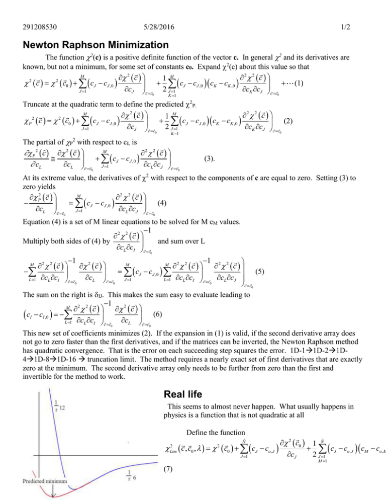
291208530
5/28/2016
1/2
Newton Raphson Minimization
The function 2(c) is a positive definite function of the vector c. In general 2 and its derivatives are
known, but not a minimum, for some set of constants c0. Expand 2(c) about this value so that
M
 2  c  
2  2 c  
1 M
 2  c    2  c0     cJ  cJ ,0 

c

c
c

c

  J J ,0  K K ,0  c c   (1)
cJ c c 2 J 1
J 1
K
J c  c
0
0
K 1
Truncate at the quadratic term to define the predicted 2P.
M
 2  c  
2  2 c  
1 M
 P 2  c    2  c0     cJ  cJ ,0 

c

c
c

c

  J J ,0  K K ,0  c c  (2)
cJ c c 2 J 1
J 1
K
J c  c
0
0
K 1
The partial of P2 with respect to cL is
M
 P 2  cˆ   2  c  
2  2 c  


c

c

  J J ,0  c c 
 cL
cL c c J 1
L
J c c
0
(3).
0
At its extreme value, the derivatives of  with respect to the components of c are equal to zero. Setting (3) to
zero yields
M
 P2  c  
2  2 c  

   cJ  cJ ,0 

 (4)
cL c c
cL cJ c c
J 1
0
0
Equation (4) is a set of M linear equations to be solved for M cM values.
1
2  2 c  
Multiply both sides of (4) by
and sum over L

cL cI c c
0
1
1 2 2

M
M
M
2  2 c  
 2  c  
2  2 c  
  c  

   cJ  cJ ,0  
(5)



cL c c J 1
cL cJ 
L 1 cL cI  c  c
L 1 cL cI  c  c
0
0
0
c c0
The sum on the right is IJ. This makes the sum easy to evaluate leading to
1
M
 2  2  c    2  c  
 cI  cI ,0    c c 
 (6)
cL c c
L 1
L
I c  c
0
0
This new set of coefficients minimizes (2). If the expansion in (1) is valid, if the second derivative array does
not go to zero faster than the first derivatives, and if the matrices can be inverted, the Newton Raphson method
has quadratic convergence. That is the error on each succeeding step squares the error. 1D-11D-21D41D-81D-16  truncation limit. The method requires a nearly exact set of first derivatives that are exactly
zero at the minimum. The second derivative array only needs to be further from zero than the first and
invertible for the method to work.
2
Real life
This seems to almost never happen. What usually happens in
physics is a function that is not quadratic at all
Define the function
Nˆ
2
 Lim
 c , c0 ,     2  c0     cJ  co, J 
J 1
(7)
 2  c0  1 Nˆ
   cJ  co, J  cM  co,M
cJ
2 J 1
M 1
291208530
5/28/2016
2/2
2
This is P , equation (1), plus a Marquardt parameter  multiplying the sum of the changes in the constants
weighted by the relative importance of the constant SJ2. For reference in the function
3
3

x  c3  
x  c3 
f A  c1 , c2 , c3 , x   c1 1 
 1 

c2  
c2  

S1  1
(8)
S2  100
S3  10000
Minimize 2p following the steps that led from (1) to (6). Setting the first derivative to zero yields
M
 Lim 2  cˆ, c0 ,    2  c  
2  2 c  
2

    cJ  cJ ,0 
  2S L  cL  cL ,0  (9)
 cL
cL c c J 1
cL cJ c c
0
0
Move the last term inside the summation
 2  2 c  

M
 Lim 2  cˆ, c0 ,    2  c  
2

    cJ  cJ ,0  
  2 S L LJ  (10)
 cL
cL c c J 1
 cL cJ c c

0


The Marquardt parameter  is a one dimensional parameter that can be found to make 2p have “almost” any
desired value. The smoothers which are to be experientially found make this multidimensional.
1. For  = 0, this is the Newton Raphson equation with all of its faults.
2. For  = infinity, the inverse of the second derivative array is zero, and the c which minimizes equation
(7) is simply c0
3. For a sufficiently large value of , the inverse can always be found.
The usual situation is shown as a one-dimensional plot on the left.
The term 2 and all of its derivatives has been evaluated at the
position c0. The expansion of 2p(c,=0) predicts a minimum at cq
which when tested is much larger than the current value of 2(c0).
The plot of 2m is also shown for a fairly large value of  which
results in cm that gives rise to a 2 which is slightly smaller than the
2(c0), but nothing to write home about. The goal of course is to find
just the right value of  so that the minimum is at cb that is also at the
minimum of 2.
0
The general method
The idea is to request an improvement in 2 by a specific amount. In particular to solve for a  such that
  p2  c    

 Fr   0 (11)

2
   c0 



The value of Fr is determined experientially. That is it is initially specified in the direction file as for example
0.99999. Then when 2 at c() is equal to the predicted value it is cubed. When it is not equal, Fr moves ¾ of
the distance towards one. Equation (11) is solved by Bracketing.doc followed by a one dimensional Newton’s
( method.