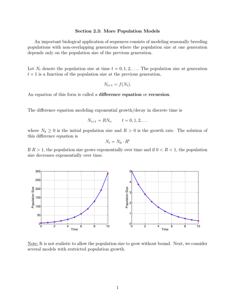
Section 2.3: More Population Models
An important biological application of sequences consists of modeling seasonally breeding
populations with non-overlapping generations where the population size at one generation
depends only on the population size of the previous generation.
Let Nt denote the population size at time t = 0, 1, 2, . . .. The population size at generation
t + 1 is a function of the population size at the previous generation,
Nt+1 = f (Nt ).
An equation of this form is called a difference equation or recursion.
The difference equation modeling exponential growth/decay in discrete time is
Nt+1 = RNt ,
t = 0, 1, 2, . . .
where N0 ≥ 0 is the initial population size and R > 0 is the growth rate. The solution of
this difference equation is
Nt = N0 · Rt
If R > 1, the population size grows exponentially over time and if 0 < R < 1, the population
size decreases exponentially over time.
300
5
4
Population Size
Population Size
250
200
150
100
2
1
50
0
0
3
2
4
6
8
0
0
10
Time
2
4
6
8
10
Time
Note: It is not realistic to allow the population size to grow without bound. Next, we consider
several models with restricted population growth.
1
The Beverton-Holt Model
The Beverton-Holt model is given by the difference equation
Nt+1 =
RNt
1 + R−1
Nt
K
where R > 1 is the growth rate and K > 0 is the carrying capacity of the population.
Example: Find all equilibria of the Beverton-Holt model and discuss their stability.
R=1.5, K=20
35
Population Size
30
25
20
15
10
5
0
0
5
10
Time
15
20
2
The Discrete Logistic Model
The discrete logistic model is given by the difference equation
Nt
Nt+1 = Nt 1 + R 1 −
K
where R > 0 is the growth rate and K > 0 is the carrying capacity of the population.
Example: Find all equilibria of the discrete logistic model and discuss their stability.
R=1.9, K=20
R=2.5, K=20
35
30
30
30
25
25
25
20
15
10
20
15
10
5
5
0
0
0
0
5
10
Time
15
20
Population Size
35
Population Size
Population Size
R=0.5, K=20
35
20
15
10
5
5
10
Time
3
15
20
0
0
5
10
Time
15
20
Note: The discrete logistic model can be simplified by rewriting the difference equation in
canonical form. The canonical form of the discrete logistic model is
xt+1 = rxt (1 − xt )
R
where xt = K(1+R)
Nt and r = 1 + R > 1. The advantage is that this difference equation is
simpler, involves only one parameter, and the variable xt ∈ (0, 1) is dimensionless.
Example: Find all equilibria of the canonical form of the discrete logistic model and discuss
their stability.
Note: If the initial population size and growth rate are not restricted, the discrete logistic
model may result in negative population sizes.
4
The Ricker Logistic Model
The Ricker logistic model is given by the difference equation
Nt
Nt+1 = Nt exp R 1 −
K
where R > 0 is the growth rate and K > 0 is the carrying capacity of the population.
Example: Find all equilibria of the Ricker logistic model and discuss their stability.
R=0.5, K=20
R=1.9, K=20
35
35
30
30
25
25
R=2.8, K=20
50
20
15
10
Population Size
Population Size
Population Size
40
20
15
10
30
20
10
5
0
0
5
5
10
Time
15
20
0
0
5
10
Time
5
15
20
0
0
5
10
Time
15
20