18.085 HOMEWORK 4 SOLUTIONS 2.2.7. Computing numerically, λ rad.
advertisement
18.085 HOMEWORK 4 SOLUTIONS
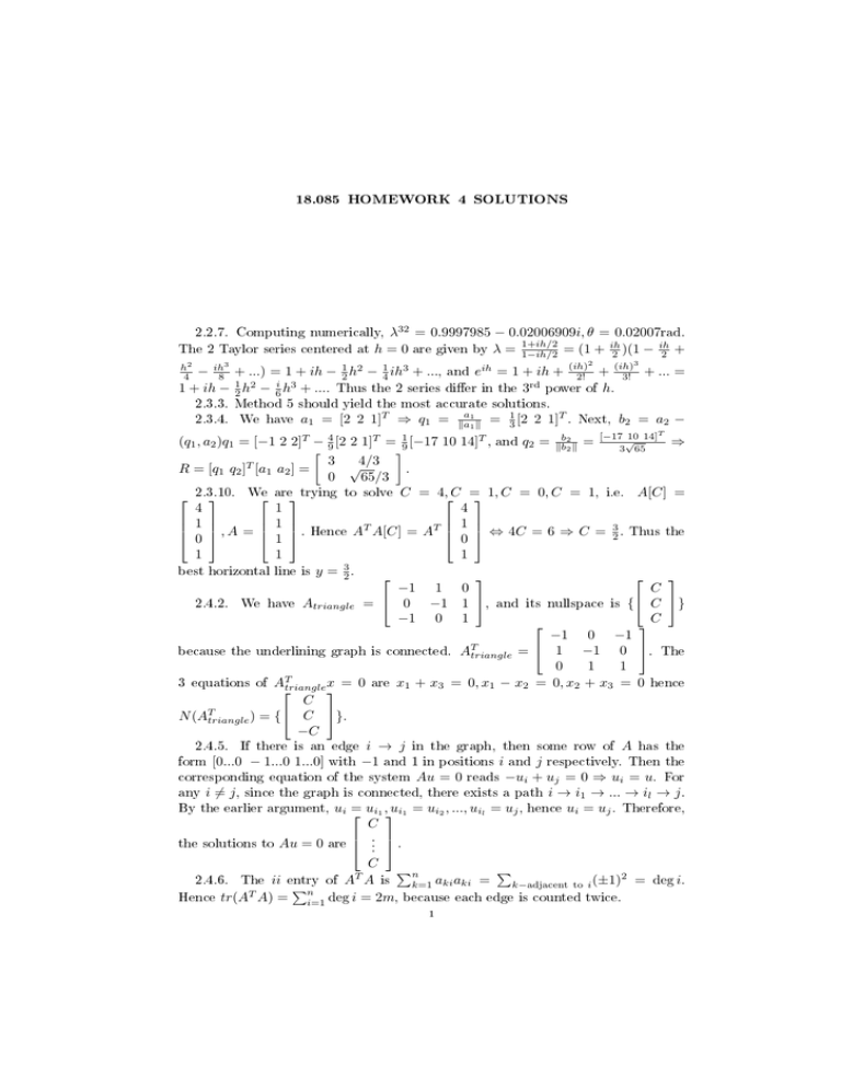
2.2.7. Computing numerically, λ32 = 0.9997985 − 0.02006909i, θ = 0.02007rad.
1+ih/2
ih
The 2 Taylor series centered at h = 0 are given by λ = 1−ih/2
= (1 + ih
2 )(1 − 2 +
2
3
3
2
(ih)
ih
1 2
1 3
h
ih
= 1 + ih + (ih)
4 − 8 + ...) = 1 + ih − 2 h − 4 ih + ..., and e
2! + 3! + ... =
i 3
1 2
1 + ih − 2 h − 6 h + .... Thus the 2 series dier in the 3rd power of h.
2.3.3. Method 5 should yield the most accurate solutions.
2.3.4. We have a1 = [2 2 1]T ⇒ q1 = kaa11 k = 13 [2 2 1]T . Next, b2 = a2 −
T
(q1 , a2 )q1 = [−1 2 2]T − 49 [2 2 1]T = 19 [−17 10 14]T , and q2 = kbb22 k = [−173√106514] ⇒
R = [q1 q2 ]T [a1 a2 ] =
3
0
√4/3
65/3
.
We
are trying to solve C = 4,C = 1, C = 0, C = 1, i.e. A[C] =
2.3.10.
4
1
4
1
, A = 1 . Hence AT A[C] = AT 1 ⇔ 4C = 6 ⇒ C = 3 . Thus the
2
0
1
0
1
1
1
best horizontal line is y = 32 .
−1 1 0
C
2.4.2. We have Atriangle = 0 −1 1 , and its nullspace is { C }
−1 0 1
C
−1 0 −1
because the underlining graph is connected. ATtriangle = 1 −1 0 . The
0
1
1
3 equations of ATtriangle
x = 0 are x1 + x3 = 0, x1 − x2 = 0, x2 + x3 = 0 hence
C
N (ATtriangle ) = { C }.
−C
2.4.5. If there is an edge i → j in the graph, then some row of A has the
form [0...0 − 1...0 1...0] with −1 and 1 in positions i and j respectively. Then the
corresponding equation of the system Au = 0 reads −ui + uj = 0 ⇒ ui = u. For
any i 6= j , since the graph is connected, there exists a path i → i1 → ... → il → j .
By the earlier argument, ui =
ui1 ,ui1 = ui2 , ..., uil = uj , hence ui = uj . Therefore,
C
..
the solutions to Au = 0 are . .
C
P
P
2.4.6. The ii entry of A A is nk=1 aki aki = k−adjacent to i (±1)2 = deg i.
P
Hence tr(AT A) = ni=1 deg i = 2m, because each edge is counted twice.
T
1
18.085 HOMEWORK 4 SOLUTIONS
0 1
0 1 , hence
−1 1
c1
0
0
0
c
0
2
A =
0
0
c3
c3
−c1 −c2 −c3
−1
2.4.7. We have A = 0
0
K = AT
c1
c2
2
0
−1
0
−c1
−c2
−c3
c1 + c2 + c3
Grounding node 4 means deletingthe 4th column
of A, hence deleting the last row
c1
0
0 , det K = c1 c2 c3 (c1 + c2 + c3 ).
0
c3
1 −1 0
0
0
−1 1
0
0 0
−1 2 −1 0
0
0 −1 1
0 0
T
, A A = 0 −1 2 −1 0
2.4.9. We have A =
.
0
0 −1 1 0
0
0 −1 2 −1
0
0
0 −1 1
0
0
0 −1 1
−1 1
0
0
−1 2 −1 0
Removing row 5 and column 5 of AT A gives (AT A)red = K =
0 −1 2 −1 =
0
0 −1 2
4 3 2 1
3 3 2 1
T4 , hence K −1 =
2 2 2 1 . Using Matlab, one nds the eigenvalues of K
1 1 1 1
to be 1, 0.1206, 2.3473, 3.5321, and det K = 1.
and column of K . Thus, Kred = 0
0
c2
0
