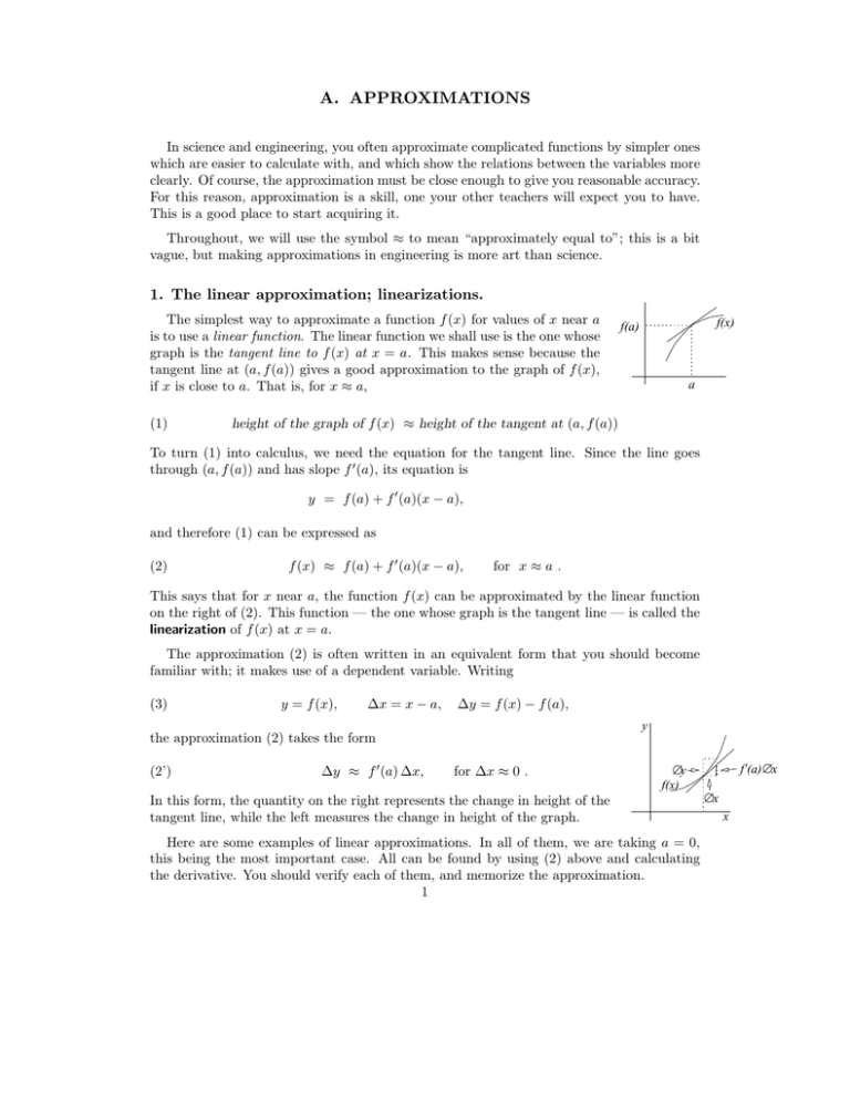
A. APPROXIMATIONS
In science and engineering, you often approximate complicated functions by simpler ones
which are easier to calculate with, and which show the relations between the variables more
clearly. Of course, the approximation must be close enough to give you reasonable accuracy.
For this reason, approximation is a skill, one your other teachers will expect you to have.
This is a good place to start acquiring it.
Throughout, we will use the symbol ≈ to mean “approximately equal to”; this is a bit
vague, but making approximations in engineering is more art than science.
1. The linear approximation; linearizations.
The simplest way to approximate a function f (x) for values of x near a
is to use a linear function. The linear function we shall use is the one whose
graph is the tangent line to f (x) at x = a. This makes sense because the
tangent line at (a, f (a)) gives a good approximation to the graph of f (x),
if x is close to a. That is, for x ≈ a,
(1)
f(x)
f(a)
a
height of the graph of f (x) ≈ height of the tangent at (a, f (a))
To turn (1) into calculus, we need the equation for the tangent line. Since the line goes
through (a, f (a)) and has slope f ′ (a), its equation is
y = f (a) + f ′ (a)(x − a),
and therefore (1) can be expressed as
(2)
f (x) ≈ f (a) + f ′ (a)(x − a),
for x ≈ a .
This says that for x near a, the function f (x) can be approximated by the linear function
on the right of (2). This function — the one whose graph is the tangent line — is called the
linearization of f (x) at x = a.
The approximation (2) is often written in an equivalent form that you should become
familiar with; it makes use of a dependent variable. Writing
(3)
y = f (x),
∆x = x − a,
∆y = f (x) − f (a),
the approximation (2) takes the form
(2’)
∆y ≈ f ′ (a) ∆x,
for ∆x ≈ 0 .
y
∆y
f(x)
In this form, the quantity on the right represents the change in height of the
tangent line, while the left measures the change in height of the graph.
Here are some examples of linear approximations. In all of them, we are taking a = 0,
this being the most important case. All can be found by using (2) above and calculating
the derivative. You should verify each of them, and memorize the approximation.
1
f (a) ∆ x
∆x
x
2
A. APPROXIMATIONS
Basic Linear Approximations
(4)
(5)
(6)
1
≈ 1 + x,
1−x
(1 + x)r ≈ 1 + rx,
for x ≈ 0 ;
for x ≈ 0 ;
sin x ≈ x,
r is any real number
for x ≈ 0 .
Note that (4) becomes a special case of (5) if we take r = −1 and replace x by −x;
nonetheless, learn (4) separately since it is very common. As an example of verification, let
us check (5):
f (x) = (1 + x)r
⇒
⇒
f ′ (x) = r(1 + x)r−1 ,
for any real r ;
′
f (0) = r .
Therefore, (2) becomes
(1 + x)r ≈ f (0) + f ′ (0) x
≈ 1+rx ,
which is (5).
2. The algebraic viewpoint; examples
Though the three basic approximations given above can be derived by using differentiation, many people remember them better by relating them to high school algebra and
geometry. We show how.
The approximation (4) can be thought of as coming from the formula for the sum of a
geometric series (memorize this too, if you have forgotten it):
1
= 1 + x + x2 + . . . + xn + . . . ,
1−x
|x| < 1 .
If x is small, then the terms x2 , x3 , . . . on the right are all negligible compared with the
term x, so they can be ignored, and we get (4).
Similarly, the approximation (5) can be thought of as coming from the binomial theorem,
if r is a positive integer:
(1 + x)r = 1 + rx +
r(r − 1) 2
x + . . . + xr .
2
As before, if x is small, we can neglect the terms in x2 , x3 , . . . , and we get the approximation
(5). Even if r is not an integer, you will learn when you study infinite series that the binomial
theorem is still formally true. Though it gives an infinite sum on the right, instead of a
finite sum, the coefficients are still calculated by the same formulas.
Finally, the linear approximation (6) for sin x should make sense if you
think of the trigonometric definition of sin x. Referring to the picture, it
says that a small arc 2x of the unit circle is approximately equal in length
to the chord 2 sin x it subtends.
1
sin x
x
A. APPROXIMATIONS
3
Continuing this algebraic viewpoint, many other linear approximation formulas can be
derived from the basic ones above by using algebra, rather than by going back to (2) and
calculating derivatives. Here are some examples of this.
Example 1. In each of the following, we want a linear approximation valid for x ≈ 0.
Observe in the first two how the variable is divided by a number (or “scaled”, as one says,
since it amounts to a change of scale or change of units for the variable). The purpose is to
put the expression in a form where one of the basic approximations can be used.
x
1/2
1
1
(a)
1−
,
by scaling and using (4);
=
≈
2+x
1 + x/2
2
2
√ p
√
(b)
9 + t = 9 1 + t/9 = 3(1 + t/9)1/2 ,
by scaling;
≈ 3(1 + t/18) = 3 + t/6,
for t ≈ 0, by using (5) .
d√
1
.
Example (b) above is just as easy to do by using (2), since
9 + t
=
dt
6
t=0
In example (c) below, however, using (2) would definitely require more work.
(c)
2+x
2+x
√
≈
≈ (2 + x)(1 − x/2), using (5), then (4);
1 + x/2
1+x
≈ 2,
multiplying out and neglecting terms in x2 .
Notice that in this example, the linearization 2 + 0 x turns out to be a constant function.
Approximations for x ≈ a, where a 6= 0 .
Though it is most common to work near a = 0, sometimes one wants another value of a.
Either one can use the formula (2), or else one can make a change of variable: h, ∆x, ǫ are
all common choices, related to x by
(7)
x = a + h,
x = a + ∆x,
x=a+ǫ .
The new variable is then close to 0 when x is close to a. Here is an example.
Example 2. Approximate 3 + x4 for x ≈ 1.
Solution. Either use (2), or change variable; doing the latter, we put x = 1 + h. Then
3 + x4 = 3 + (1 + h)4 ,
≈ 3 + (1 + 4h),
≈ 4 + 4(x − 1),
h ≈ 0,
using (5);
for x ≈ 1.
Applications. Here are a few typical uses of the linearization.
Example 3. In the theory of special relativity, the mass m of a body moving with speed
v is given by
m = √
m0 c
,
c2 − v 2
m0 = mass at rest, c = velocity of light
What speed produces a 1% increase in mass?
4
A. APPROXIMATIONS
Solution. We could crank out the answer, using the formula for m, but in practise a
simplifying approximation would be used. To begin with, scale m and v, i.e., divide them
by suitable constants to make them dimensionless: m/m0 and v/c; this turns the above
formula into (dividing top and bottom by c):
1
1
m
= p
,
=
2
2
m0
(1 − u2 )1/2
1 − v /c
where we have set v/c = u; when v is small compared with c, then u ≈ 0. We get, using (5)
with r = 1/2,
1
1
u2
≈
≈ 1+ ,
u ≈ 0,
2
2
1/2
1 − (1/2)u
2
(1 − u )
where the second approximation used (4), with x = u2 /2.
This approximation shows that to make m/m0 = 1.01 (this represents a 1% increase in
the mass), we want
√
u2 /2 = .01,
i.e.,
u = .02 ≈ 1/7 .
The corresponding velocity is (remember that u = v/c):
v ≈ c/7 ≈ (186, 000/7 mi/sec ≈ 27, 000 mi/sec.
Example 4. Give a useful approximate formula, valid for relatively small heights,
showing how the weight of a body decreases as it rises above the earth, and use your
formula to determine how high it must rise to experience a 1% loss in weight.
Solution. Let R be the radius of the earth. The force between two masses m1 and M2
with centers of mass separated by a distance d is
F =
Gm1 m2
,
d2
so if the earth weight is M and our body has weight m,
GM m
R2
GM m
,
so that
weight at height h above surface =
(R + h)2
1
R2
weight at height h
=
,
=
2
weight at surface
(R + h)
(1 + h/R)2
weight at surface =
where in this last step we made the variable dimensionless by dividing numerator and
denominator by R2 ; this scaling also makes the expression simpler. We continue with
approximations:
≈ (1 − h/R)2 ,
≈ 1 − 2h/R,
using (4);
using (5).
The approximation is valid if h/R ≈ 0, i.e., if h is very small compared to R.
A. APPROXIMATIONS
5
Using our approximation, we see that to make the ratio of the weights ≈ .99, we want
2h
= .01,
R
i.e.,
h =
.01R
.01 · 4, 000
=
= 20 miles.
2
2
4. Quadratic approximations.
To get greater accuracy, sometimes one wants to include higher-order terms in the approximating function. If we include second-order terms — that is, terms in (x − a)2 , we get
what is called a quadratic approximation for x ≈ a. It looks like
f (x) ≈ A + B(x − a) + C(x − a)2 ,
(8)
x≈a.
There is a general formula for the coefficients A, B, C using calculus, but let’s work algebraically first, and consider the basic approximations.
Basic Quadratic Approximations
(9)
(10)
(11)
1
≈ 1 + x + x2 ,
1−x
r(r − 1) 2
(1 + x)r ≈ 1 + rx +
x ,
2
sin x ≈ x,
2
(12)
cos x ≈ 1 −
x
,
2
for x ≈ 0 ;
for x ≈ 0 ;
r is any real number
for x ≈ 0 .
for x ≈ 0 .
Discussion
Formula (9) comes as before from the sum of the geometric series.
Formula (10) is the beginning of the binomial theorem, if r is an integer.
Formula (11) looks like our earlier linear approximation, but the assertion here is that it
is also the best quadratic approximation — that is, the term in x2 has 0 for its coefficient.
This is so because sin x is an odd function, so the approximating polynomial should be odd
also, which means it cannot have any x2 term.
Formula (12) is derived from (11) and the identity sin2 x + cos2 x = 1; this is one of the
exercises.
Using these basic quadratic approximations, we can by algebra get quadratic approximations to more involved expressions. Examples are given below. In studying the examples,
notice that during the course of the calculation, all approximations must be quadratic. If
one of the approximations you use is only linear, then that contaminates the final result,
which probably will not have the correct x2 term. This is the same principle you meet in
adding numbers: if one of the numbers is only good to one decimal place, then no matter
how accurate all the other numbers are, the sum will only be good to one decimal place.
6
A. APPROXIMATIONS
Example 5. By using the basic approximations, give quadratic approximations valid
for x ≈ 0 for each of the following:
√
√
cos x
(d)
(a) sec x
(b)
1 + 3x
(c)
1 + x + x2
1−x
Solution.
(a)
(b)
(c)
sec x =
1
x2
1
≈
≈ 1+ ,
2
cos x
1 − x /2
2
by (12) and (4).
√
1
1
1 + 3x = (1 + 3x)1/2 ≈ 1 + (3x) − (3x)2 ,
2
8
3
9
≈ 1 + x − x2 .
2
8
by (10);
1/2
1 + (x + x2 )
1
1
3
1
≈ 1 + (x + x2 ) − (x + x2 )2 ≈ 1 + x + x2 ,
2
8
2
8
p
1 + x + x2 =
cos x
≈
1−x
(d)
by (10).
x2
x2
(1 + x + x2 ) ≈ 1 + x +
1−
.
2
2
To illustrate what happens if you don’t keep enough terms during the calculation, observe
that if in (d) above we only used 1 + x in the right-hand factor, the answer would have been
1 + x − x2 /2, whose x2 term is incorrect.
6. The quadratic approximation formula.
(13)
f (x) ≈ f (a) + f ′ (a)(x − a) +
f ′′ (a)
(x − a)2 ,
2
for x ≈ a.
Example 6. Check formulas (10) and (11) by using (13).
Solution. Since the first two terms of (13) are the linearization, we can build on our earlier
work, and have only to calculate the quadratic coefficient f ′′ (0)/2. We get
(a)
sin x ≈ 0 + x + 0x2 ,
since sin′′ (x) = − sin x
⇒
sin′′ (0) = 0.
(b)
f (x) = (1 + x)r
⇒
f ′′ (x) = r(r − 1)(1 − x)r−2
⇒
r(r − 1)
f ′′ (0)
=
,
2
2
as in (10).
The usefulness of (13) is tempered by the fact that it requires calculation of second
derivatives. This can get rather tedious — function (d) in Example 5 is a good illustration
— so that using the algebraic techniques is often better.
A. APPROXIMATIONS
7
The quadratic approximation formula (13) may be “derived” as follow. We are looking
for the right choice of coefficients in
(14)
f (x) ≈ A + B(x − a) + C(x − a)2 ,
x ≈ a.
Let us denote by Q(x) the polynomial on the right of (14). Then it makes sense to choose
the coefficients A, B, C so that f (x) and Q(x) have the same value and the same first and
second derivatives at a, i.e., so that
(15)
f (a) = Q(a),
f ′ (a) = Q′ (a),
f ′′ (a) = Q′′ (a) .
Since Q′ (x) = B + 2C(x − a) and Q′′ (x) = 2C, equations (15) say that
(16)
f (a) = A,
f ′ (a) = B,
f ′′ (a) = 2C ;
these values for A, B, C turn (14) into (13), as promised. Note that the first two terms on
the right of (13) give the linearization at x = a; thus the quadratic approximation refines
the linear approximation by adding a quadratic term to it.
Exercises: Section 2A