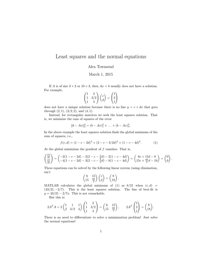
Least squares and the normal equations
Alex Townsend
March 1, 2015
If A is of size 3 × 2 or 10 × 3, then Ax = b usually does not have a solution.
For example,


 
1 2
1
1 3/2 c = 2
d
1 4
1
does not have a unique solution because there is no line y = c + dx that goes
through (2, 1), (3/2, 2), and (4, 1).
Instead, for rectangular matrices we seek the least squares solution. That
is, we minimize the sum of squares of the error
kb − Axk22 = (b − Ax)21 + . . . + (b − Ax)2n .
In the above example the least squares solution finds the global minimum of the
sum of squares, i.e.,
f (c, d) = (1 − c − 2d)2 + (2 − c − 3/2d)2 + (1 − c − 4d)2 .
(1)
At the global minimium the gradient of f vanishes. That is,
! ∂f
6c + 15d − 8
−2(1 − c − 2d) − 2(2 − c − 32 d) − 2(1 − c − 4d)
0
∂c
=
=
=
.
∂f
0
d
−
18
15c + 89
−4(1 − c − 2d) − 3(2 − c − 32 d) − 8(1 − c − 4d)
2
∂c
These equations can be solved by the following linear system (using elimination,
say):
6 15
c
8
=
.
d
18
15 89
2
MATLAB calculates the global minimum of (1) as 8/21 when (c, d) =
(43/21, −2/7). This is the least squares solution. The line of best-fit is
y = 43/21 − 2/7x. This is not remarkable.
But this is:
 


1 2
1
6
15
8
1
1
1
T  
T


2 =
1 3/2 =
,
2A
2A A = 2
.
18
2 3/2 4
15 89
2
1
1 4
There is no need to differentiate to solve a minimization problem! Just solve
the normal equations!
1
NORMAL EQUATIONS:
AT Ax = AT b
Why the normal equations? To find out you will need to be slightly crazy
and totally comfortable with calculus.
In general, we want to minimize1
f (x) = kb − Axk22 = (b − Ax)T (b − Ax) = bT b − xT AT b − bT Ax + xT AT Ax.
If x is a global minimum of f , then its gradient ∇f (x) is the zero vector. Let’s
take the gradient of f remembering that

∂f
∂x1



∇f (x) =  ...  .
∂f
∂xn
We have the following three gradients:
∇(xT AT b) = AT b,
∇(bT Ax) = AT b,
∇(xT AT Ax) = 2AT Ax.
To calculate these gradients, write out xT AT b, bT Ax, and xT AT Ax, in terms
of sums and differentiate with respect to x1 , . . . , xn (this gets very messy).
Thus, we have
∇f (x) = 2AT Ax − 2AT b,
just like we saw in the example. We can solve ∇f (x) = 0 or, equivalently
AT Ax = AT b to find the least squares solution. Magic.
Is this the global minimum? Could it be a maximum, a local minimum,
or a saddle point? To find out we take the “second derivative” (known as the
Hessian in this context):
Hf = 2AT A.
Next week we will see that AT A is a positive semi-definite matrix and that this
implies that the solution to AT Ax = AT b is a global minimum of f (x). Roughly
speaking, f (x) is a function that looks like a bowl.
1 Here,
x is a vector not a 1D variable.
2