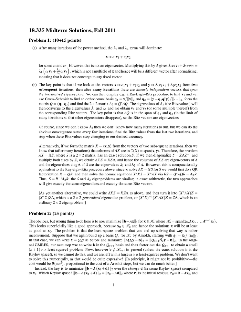
18.335 Midterm Solutions, Fall 2011
Problem 1: (10+15 points)
(a) After many iterations of the power method, the λ1 and λ2 terms will dominate:
x ≈ c1 v1 + c2 v2
forsome c1 and c2 .However, this is not an eigenvector. Multiplying this by A gives λ1 c1 v1 + λ2 c2 v2 =
λ1 c1 v1 + λλ2 c2 v2 , which is not a multiple of x and hence will be a different vector after normalizing,
1
meaning that it does not converge to any fixed vector.
(b) The key point is that if we look at the vectors x ≈ c1 v1 + c2 v2 and y ≈ λ1 c1 v1 + λ2 c2 v2 from two
subsequent iterations, then after many iterations these are linearly independent vectors that span
the two desired eigenvectors. We can then employ e.g. a Rayleigh–Ritz procedure to find v1 and v2 :
use Gram–Schmidt to find an orthonormal basis q1 = x/kxk2 and q2 = (y − q1 q∗1 y) /k · · · k2 , form the
matrix Q = (q1 , q2 ) and find the 2 × 2 matrix A2 = Q∗ AQ. The eigenvalues of A2 (the Ritz values) will
then converge to the eigenvalues λ1 and λ2 and we obtain v1 and v2 (or some multiple thereof) from
the corresponding Ritz vectors. The key point is that AQ is in the span of q1 and q2 (in the limit of
many iterations so that other eigenvectors disappear), so the Ritz vectors are eigenvectors.
Of course, since we don’t know λ3 then we don’t know how many iterations to run, but we can do the
obvious convergence tests: every few iterations, find the Ritz values from the last two iterations, and
stop when these Ritz values stop changing to our desired accuracy.
Alternatively, if we form the matrix X = (x, y) from the vectors of two subsequent iterations, then we
know that (after many iterations) the columns of AX are in C(X) = spanhx, yi. Therefore, the problem
AX = XS, where S is a 2 × 2 matrix, has an exact solution S. If we then diagonalize S = ZΛZ −1 and
multiply both sizes by Z, we obtain AXZ = XZΛ, and hence the columns of XZ are eigenvectors of A
and the eigenvalues diag Λ of S are the eigenvalues λ1 and λ2 of A. However, this is computationally
equivalent to the Rayleigh–Ritz procedure above, since to solve AX = XS for S we would first do a QR
factorization X = QR, and then solve the normal equations X ∗ XS = X ∗ AX via RS = Q∗ AQR = A2 R.
Thus, S = R−1 A2 R: the S and A2 eigenproblems are similar; in exact arithmetic, the two approaches
will give exactly the same eigenvalues and exactly the same Ritz vectors.
[As yet another alternative, we could write AXZ = XZΛ as above, and then turn it into (X ∗ AX)Z =
(X ∗ X)ZΛ, which is a 2 × 2 generalized eigenvalue problem, or (X ∗ X)−1 (X ∗ AX)Z = ZΛ, which is an
ordinary 2 × 2 eigenproblem.]
Problem 2: (25 points)
The obvious, but wrong thing to do here is to now minimize kb−Axk2 for x ∈ Kn where Kn = spanhx0 , Ax0 , . . . , An−1 x0 i.
This looks superficially like a good approach, because x0 ∈ Kn and hence the solutions x will be at least
as good as x0 . The problem is that the least-square problem that you end up solving that way is rather
inconvenient. Suppose that we again build up a basis Qn for Kn by Arnoldi, starting with q̃1 = x0 /kx0 k2 .
In that case, we can write x = Qn y as before and minimize kAQn y − bk2 = kQn+1 H̃n y − bk2 . In the original GMRES, our next step was to write b in the Qn+1 basis and then factor out the Qn+1 to obtain a small
(n + 1) × n least-squared problem. Now, however b ∈
/ Kn+1 in general (unless the exact solution is in the
Krylov space!), so we cannot do this, and we are left with a huge m×n least-squares problem. We don’t want
to solve this numerically, as that would be quite expensive! [In principle, it might not be prohibitive—the
cost would be θ (mn2 ), proportional to the cost of n Arnoldi steps, but we can do much better.]
Instead, the key is to minimize kb − A (x0 + d) k2 over the change d (in some Krylov space) compared
to x0 . Which Krylov space? kb−A (x0 + d) k2 = kr0 −Adk2 where r0 is the initial residual r0 = b−Ax0 , and
1
from above we need r0 to be ∈ K˜n to simplify our least-squares problem, so we want K˜n = spanhr0 , Ar0 , . . . , An−1 r0 i .
That is, we start our Arnoldi process with q̃1 = r0 /kr0 k2 to build up our orthonormal basis Qn for our new
K˜n , and then write d = Qn y. Now, since r0 = Qn+1 r0 e1 where r0 = kr0 k, we obtain a small least-squares
problem min kH̃n y − r0 e1 k2 that we can solve for y and hence obtain solutions x = x0 + Qn y . Since these
y
again contain x0 , they clearly must be improvements on the solution when we minimize the residual over all
y.
Problem 3: (15+10 points)
(a) Solutions:
h
i h
i
kxk
(i) Consider κ(B) = maxx6=0 kBxk
kxk · maxx6=0 kBxk . Since B is the first p columns of A, for any
 
x
 0 
x we can write Bx = Ax0 where x0 =   just has extra zero components to multiply the
..
.
columns > p of A by zero. Note that kxk = kx0 k in the L2 norm that we usually use for κ (and
for that matter would be true in most typical norms). Hence
max
x6=0
kBxk
kAx0 k
kAxk
= max
≤ max
kxk
x6=0 kx0 k
x6=0 kxk
since the vectors x0 are a subset of all vectors in Cn . Similarly for
as desired.
kxk
kBxk
. Therefore κ(B) ≤ κ(A)
(ii) In a data-fitting problem, adding columns to the matrix corresponds to increasing the number
of degrees of freedom, which in this case means increasing the degree of the polynomial.
Hence, increasing the degree of the polynomial increases the sensitivity of the fit coefficients
to experimental errors (recall that condition numbers bound the ratio of relative errors in the
output to relative errors in the input).
(b) If κ(A) is finite then A has full column rank. Write the reduced SVD A = Û Σ̂V̂ ∗ where Û is m × n, Σ̂
is the n × n diagonal matrix of the n singular values, and V̂ is n × n. κ(A) = 1 implies σmin = σmax ,
which means that all the singular values are equal to some value σ and Σ̂ = σ I is a multiple of the
n × n identity matrix. Hence A = σ Û V̂ ∗ = σ Q where Q = Û V̂ ∗ satisfies Q∗ Q = V̂
Û ∗
Û V̂ ∗ = V̂ V̂ ∗ = I
(noting that V̂ is square hence unitary). Therefore A = cQ with c = σ and Q = Û V̂ ∗ .
Problem 4: (8+8+9 points)
(a) The problem is that large xpor large y (magnitude & 10154 ) can cause x2 or y2 to overflow and give
∞, even though the result x2 + y2 should be in a representable range. This fix is simple: let z =
max(|x|, |y|) (which can be computed without multiplications or danger of overflow), and write
q
p
p
2
2
x + y = z (x/z)2 + (y/z)2 ≈ z ⊗ (x z) ⊗ (x z) ⊕ (y z) ⊗ (y z).
Since we are now multiplying rescaled numbers with magnitudes ≤ 1, there is no danger of overflow
and we can expect an accurate result for all representable numbers.
√
(b) The problem with x = −b ± b2 − 1 is that for very large b, if b2 > 1/εmachine then b2 1 will give
√
^
2
b2 , and
√one of the two roots will have extremely large relative error. Say b > 0, then −b + b − 1 ≈
−b ⊕ b ⊗ b will be all roundoff errors.
2
One way to fix this is to check for the case of large |b| and to Taylor-expand the second root in
qthat case.
√
1 2
1
3
1 + z = 1 + 2 z − 8 z + O(z ), so the problematic root can be approximated by −b + b 1 − b12 =
1
−b + b 1 − 2b12 − 8b14 + O(b−6 ) ≈ − 2b
− 8b13 . This will give us a much more accurate answer.
The next-order term in the Taylor expansion would be −bz3 /16 = −1/16b5 , or a relative error
5
1
≈ 1/16b
1/2b = 8b4 , which is less that εmachine in double precision for |b| & 5000. So, we can use
the two-term Taylor expansion to get extremely accurate answers as soon as |b| > 5000, and use the
exact expression otherwise.
Another, even nicer solution, is to use the fact√
that the product of the two roots is 1, so we√can in1
√
(switching to −b + · · · for
stead write the two roots (for b > 0) as −b − b2 − 1 and
2
−b−
b −1
b < 0), which are exact expressions that suffer no cancellation problems for large |b|.
A separate but less dramatic problem occurs for b = ±1 + δ where |δ | is very small (as can be
seen by taking the derivative with b, the condition numbers of both roots diverge as δ → 0). Suppose
2
|δ | ∼ εmachine and b = 1 + δ . Then b ⊗ b 1 ≈ 2δ + ε4 + O(εmachine
) where |ε4 | ≤ 4εmachine
2
(where√the 4 comes from combining the
√ various ε factors 2for different operations in b − 1). Then
2
−b + b − 1 is computed as −1 − δ + 2δ + ε4 + ε + O(εmachine ) where |ε| ≤ 4εmachine , and the
√
√
√
error (both absolute and relative) is 2δ + ε4 − 2δ + O(εmachine ) = O( εmachine ). So, although
the error is not large in absolute terms, it converges more slowly than would be required by the strict
stability criteria. Essentially, once the user computes 1 + η we are sunk since we have thrown out most
or all of the digits of η for small |η|. The only way to fix this is top
have the user specify something like
η = b − 1 instead of b, in which case we can compute 1 + η ± 2η + η 2 with O(εmachine ) errors
even for very small |η|. However, the large-|b| failure is much more dramatic and problematic.
(c) The problem is that for small |x|, cos x ≈ 1 and so 1 − cos x will suffer a large cancellation error.
One approach is to check whether |x| is small and to switch to a Taylor expansion in this case, as
in the previous problem, and that is a perfectly valid solution. Another, somewhat more elegant approach, is to use the trigonometric identity 1 − cos x = 2 sin2 (x/2), which involves no subtractive
cancellation and will give us nearly machine precision for a wide range of x. [There are various
other trig identities you could use instead, e.g. 1 − cos2 x = sin2 x = (1 − cos x)(1 + cos x) and hence
1 − cos x = sin2 x/(1 + cos x), which is accurate for small |x|, but this is more expensive than the halfangle formula.]
(Note that there is a very different problem for very large x. For very large x, evaluating cos x requires the computation of the remainder after dividing x by π. So, for example, if x = 10100 then one
would need to compute x/π to ∼ 115 decimal digits in order to evaluate cos x to machine precision.
[There is a famous story in which Paul Olum stumped Richard Feynman by posing a similar question.]
Because of this, in in practice numerical libraries only compute sin and cos accurately if you give them
angles not too much bigger than π.)
3