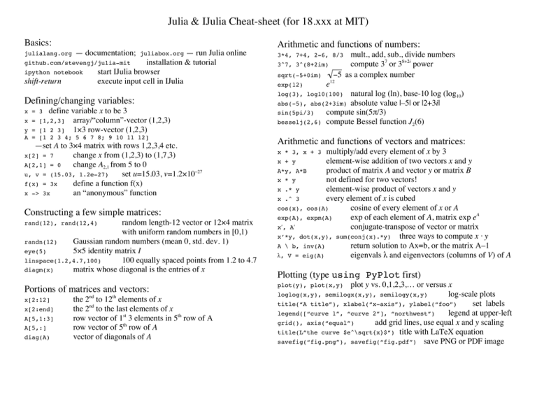
Julia & IJulia Cheat-sheet (for 18.xxx at MIT)
Basics:
— run Julia online
github.com/stevengj/julia-mit
installation & tutorial
ipython notebook
start IJulia browser
shift-return
execute input cell in IJulia
julialang.org
— documentation;
juliabox.org
Defining/changing variables:
define variable x to be 3
[1,2,3] array/“column”-vector (1,2,3)
[1 2 3] 1×3 row-vector (1,2,3)
Arithmetic and functions of numbers:
3^7, 3^(8+2im)
sqrt(-5+0im)
exp(12)
€
x =
besselj(2,6)
Constructing a few simple matrices:
random length-12 vector or 12×4 matrix
with uniform random numbers in [0,1)
randn(12)
Gaussian random numbers (mean 0, std. dev. 1)
eye(5)
5×5 identity matrix I
linspace(1.2,4.7,100)
100 equally spaced points from 1.2 to 4.7
diagm(x)
matrix whose diagonal is the entries of x
rand(12), rand(12,4)
Portions of matrices and vectors:
x[2:12]
x[2:end]
A[5,1:3]
A[5,:]
diag(A)
the 2nd to 12th elements of x
the 2nd to the last elements of x
row vector of 1st 3 elements in 5th row of A
row vector of 5th row of A
vector of diagonals of A
natural log (ln), base-10 log (log10)
absolute value |–5| or |2+3i|
compute sin(5π/3)
compute Bessel function J2(6)
abs(-5), abs(2+3im)
sin(5pi/3)
—set A to 3×4 matrix with rows 1,2,3,4 etc.
x[2] = 7
change x from (1,2,3) to (1,7,3)
A[2,1] = 0
change A2,1 from 5 to 0
u, v = (15.03, 1.2e-27)
set u=15.03, v=1.2×10–27
f(x) = 3x
define a function f(x)
x -> 3x
an “anonymous” function
e12
log(3), log10(100)
x = 3
y =
A = [1 2 3 4; 5 6 7 8; 9 10 11 12]
mult., add, sub., divide numbers
compute 37 or 38+2i power
−5 as a complex number
3*4, 7+4, 2-6, 8/3
Arithmetic and functions of vectors and matrices:
multiply/add every element of x by 3
x + y
element-wise addition of two vectors x and y
A*y, A*B
product of matrix A and vector y or matrix B
x * y
not defined for two vectors!
x .* y
element-wise product of vectors x and y
x .^ 3
every element of x is cubed
cos(x), cos(A)
cosine of every element of x or A
exp(A), expm(A)
exp of each element of A, matrix exp eA
xʹ′, Aʹ′
conjugate-transpose of vector or matrix
x’*y, dot(x,y), sum(conj(x).*y) three ways to compute x · y
A \ b, inv(A)
return solution to Ax=b, or the matrix A–1
λ, V = eig(A)
eigenvals λ and eigenvectors (columns of V) of A
x * 3, x + 3
Plotting (type using PyPlot first)
plot y vs. 0,1,2,3,… or versus x
loglog(x,y), semilogx(x,y), semilogy(x,y)
log-scale plots
title(“A title”), xlabel(“x-axis”), ylabel(“foo”)
set labels
legend([“curve 1”, “curve 2”], “northwest”)
legend at upper-left
grid(), axis(“equal”)
add grid lines, use equal x and y scaling
title(L”the curve $e^\sqrt{x}$”) title with LaTeX equation
savefig(“fig.png”), savefig(“fig.pdf”) save PNG or PDF image
plot(y), plot(x,y)