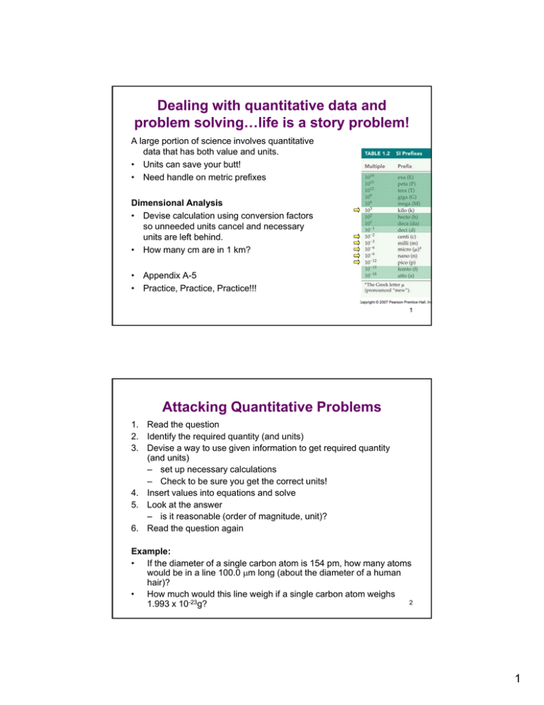
Dealing with quantitative data and
problem solving…life is a story problem!
A large portion of science involves quantitative
data that has both value and units.
• Units can save your butt!
• Need handle on metric prefixes
Dimensional Analysis
• Devise calculation using conversion factors
so unneeded units cancel and necessary
units are left behind.
• How many cm are in 1 km?
• Appendix A-5
• Practice, Practice, Practice!!!
1
Attacking Quantitative Problems
1. Read the question
2. Identify the required quantity (and units)
3. Devise a way to use given information to get required quantity
(and units)
– set up necessary calculations
– Check to be sure you get the correct units!
4. Insert values into equations and solve
5. Look at the answer
– is it reasonable (order of magnitude, unit)?
6. Read the question again
Example:
• If the diameter of a single carbon atom is 154 pm, how many atoms
would be in a line 100.0 m long (about the diameter of a human
hair)?
• How much would this line weigh if a single carbon atom weighs
2
1.993 x 10-23g?
1
What can a result tell us?
What is the "truth"?
• We don't (and can't) determine the "true value" of any component in
a mixture.
– All measurements
t h
have some associated
i t d error ((uncertainty).
t i t )
– Representation of results must illustrate this error; otherwise value is
useless!
• We can work to understand (and improve) the precision of a
measurement.
– Precision =
• Comparing multiple methods increases confidence in the accuracy
of our results.
– Accuracy =
3
Representation of Quantitative Data
Significant Figures: Number of digits necessary to present a result
with the appropriate accuracy.
– Last digit has uncertainty, at least 1!
• Results are presented to the appropriate number of significant
figures, and often accompanied by the error in the final digit.
Value  Error
e.g. 102.5  0.1 ppm
• When rounding, look at all digits beyond the last place needed.
• Always round values that are exactly halfway to the nearest even
digit.
12.250  12.2
12.350  12.4
12.250001  12.3
4
2
Guidelines for Sig. Figs.
When looking at a number:
1. all nonzero digits are significant,
2 allll zeros th
2.
thatt appear b
between
t
nonzero di
digits
it off a number
b are
significant,
3. all zeros at the end of a number on the right hand side of the
decimal point are significant,
4. all other zeros are not significant.
Examples: How many significant figures in each value?
14600
0.0146
14060.0
10460
5
Sig. Figs. and Calculations
In doing calculations, the number sig figs is limited by the least certain
piece of data.
– Addition/Subtraction
– Multiplication/Division
• Example: How many sig. figs. should be in the answers to the
following:
126.23 + 0.0147 =
58.6 x 3.1 =
• NOTE: Wait to truncate results until the end of the calculation!
WHY???
• Indicate “extra” digits by subscripting:
• Exact numbers don’t impact sig. figs.
6
3
Types of Error (Uncertainty)
•
Uncertainties fall into two main classes:
– Systematic Error:
– Random Error
•
Two general approaches to quantifying error:
– Absolute Uncertainty
– Relative Uncertainty, (% Relative Uncertainty)
7
Statistics and Quantitative Data
• Statistics allow an estimation of uncertainty in our data.
– AS LONG AS:
• Two parameters define the distribution:
 :
 :
• Statistical analyses relate experimental
data to this “ideal” distribution.
– BUT, there are some challenges!
Fre
equency of Observations
• Foundation of statistics: Normal Distribution
Observed Value
8
4
Statistics in Practice:
Remember the key assumption!
Describing the precision of our data.
• Average, or Arithmetic Mean:
– n is the number of samples
x
•
 xi
i
n
Sample Standard Deviation:
 x i  x 
2
s
i
n 1
9
Describing the “uncertainty” in our data.
How good is it?
• When we determine an average (with some associated
error), how sure are we that the "true value" is close to
this a
average?
erage?
– What factors influence this confidence?
• The most common statistical tool for determining that the
"true" value is close to our calculated mean is the
confidence interval.
– Th
The confidence
fid
iinterval
t
l presents
t a range about
b t the
th mean, within
ithi
which there is a fixed probability of finding the “true value”, m.
x
ts
n
10
5
More on Confidence Limits
• Values for t are tabulated based on several confidence levels and
various numbers of degrees of freedom.
Confidence Level (%)
Degrees of
Freedom
50
90
95
98
99
99.5
99.9
3
0.765
2.353
3.182
4.541
5.841
7.453
12.924
120
0.677
1.658
1.980
2.358
2.617
2.860
3.373
– NOTE: even though the number of measurements (n) is used in the CI
calculation, t is determined based on the degrees of freedom (n-1).
• Let’s look at some data:
What is the average?
What is the standard deviation (s)?
What is the 95% confidence limit?
4.9761
4.9693
4.9713
4.8903
4.9631
4.9551
4.9586
5.0012
4.9781
4.9895
11
Error Propagation
(aka propagation of uncertainty)
How do errors in individual values affect an analysis?
– Effects depend on how the data is used.
– “Rules”
“R l ” come ffrom calculus!
l l !
Error Propagation in Addition and Subtraction:
– Overall error is based on the absolute uncertainties of individual
values.
2
2
e 4  e1  e 2  e 3
– Example:
2
12.4  0.2
5.7  0.1
+
1.43  0.04
19.53  ???
12
6
More Error Propagation
Error Propagation in Multiplication and Division
– Concept is the same as addition and subtraction, except
relative uncertainties are used
2
2
e 
e 
e 
e4
  1    2    3 
v4
v
v
 2
 1
 v3 
%e 4 
2
%e12  %e2 2  %e3 2
13
7