Numerical Methods
MATH 417 - 501/502
A. Bonito
February 4
Spring 2016
Last Name:
First Name:
Homework 2
Exercise 1
60%
The goal of this exercise is to write a matlab code based on the Vandermonde approach to determine
the polynomial pn of degre n such that
pn (xi ) = yi ,
i = 0, ..., n
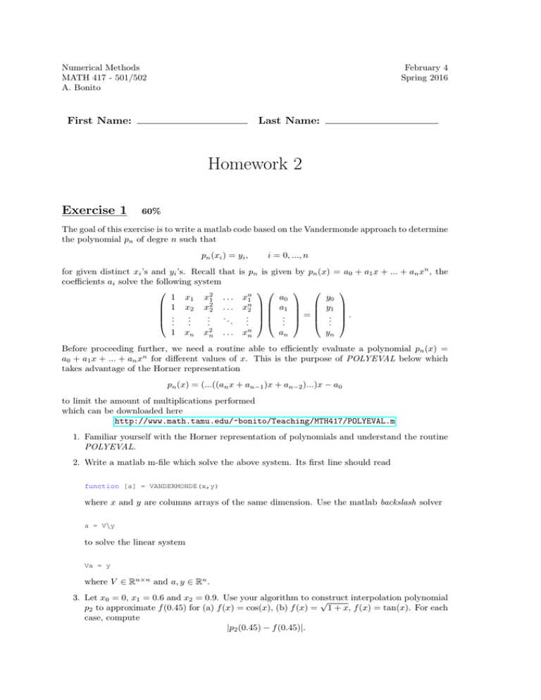
for given distinct xi ’s and yi ’s. Recall that is pn is given by pn (x) = a0 + a1 x + ... + an xn , the
coefficients ai solve the following system

 


a0
y0
1 x1 x21 . . . xn1
 1 x2 x22 . . . xn2   a1   y1 

 


 ..
..
.. . .
.  .  =  . .
 .
. ..   ..   .. 
.
.
an
yn
1 xn x2n . . . xnn
Before proceeding further, we need a routine able to efficiently evaluate a polynomial pn (x) =
a0 + a1 x + ... + an xn for different values of x. This is the purpose of POLYEVAL below which
takes advantage of the Horner representation
pn (x) = (...((an x + an−1 )x + an−2 )...)x − a0
to limit the amount of multiplications performed
which can be downloaded here
http://www.math.tamu.edu/~bonito/Teaching/MTH417/POLYEVAL.m
1. Familiar yourself with the Horner representation of polynomials and understand the routine
POLYEVAL.
2. Write a matlab m-file which solve the above system. Its first line should read
function [a] = VANDERMONDE(x,y)
where x and y are columns arrays of the same dimension. Use the matlab backslash solver
a = V\y
to solve the linear system
Va = y
where V ∈ Rn×n and a, y ∈ Rn .
3. Let x0 = 0, x1 = 0.6 and x2 = 0.9. Use your algorithm to construct
interpolation polynomial
√
p2 to approximate f (0.45) for (a) f (x) = cos(x), (b) f (x) = 1 + x, f (x) = tan(x). For each
case, compute
|p2 (0.45) − f (0.45)|.
Exercise 2
40%
This exercise explores the Runge interpolation paradox.
Consider the function
1
f (x) =
1 + 25x2
on the interval [−1, 1]. Use the following matlab commands to see how the function looks like
z = linspace(-1,1,200);
yexact = 1./(1+25.*z.ˆ2);
plot(x,yexact)
We propose to construct interpolations of this function using equally spaced interpolation points on
[−1, 1]. Given N + 1 interpolation points, define the interpolations nodes to be equally distributed
in the interval [−1, 1]
x = linspace(-1,1,N+1);
Use the matlab commands polyfit to construct the associated interpolation polynomial of degree
N (your VANDERMONDE implementation does the same job except that polyfit returns a =
(an , an−1 , ..., a1 , a0 )t )
a = polyfit(x,1./(1+25.*x.ˆ2),N);
In order to compare the interpolation polynomial with the function f , we also need to compute
the value of the interpolation polynomial at the points z defined above. To do this, you can use
the matlab command polyval
yinter = polyval(a,z);
Again, notice that polyval does the same as POLYEVAL in the previous exercise except that the coefficients a are flipped, i.e. polyval expect the coefficient in the following order a = (an , an−1 , ..., a0 )t .
This matches the output from polyfit. Finally, the commands
plot(z,yexact,z,yinter);
legend('exact','interpolation');
graph the exact function and its interpolation on the same plot.
1. Chose N = 2, 5, 10, 15, 20, 30 and graph for each case the function f and interpolation polynomial on the same plot.
2. What do you conclude? explain why using the error bound on polynomial approximations
discussed in class.
3. Instead of equi-distributed interpolation points x, define
(2j + 1)π
,
xi = −1 + 1 + cos
2(N + 1)
for i = 0, ..., N.
Perform the same computations with these points and return the corresponding graphs.
Notice where the interpolation points lie in the interval [−1, 1]. What do you conclude?
4. Instead of global interpolation, define the piecewise linear interpolant. For given N set
xi := −1 + 2i/N and defined P1N (x) on each interval [xi , xi+1 ] by
P1N (x)|[xi ,xi+1 ] := f (xi ) +
x − xi
(f (xi+1 ) − f (xi )).
xi+1 − xi
Chose N = 2, 5, 10, 15, 20, 30 and return the corresponding graphs. What do you conclude?