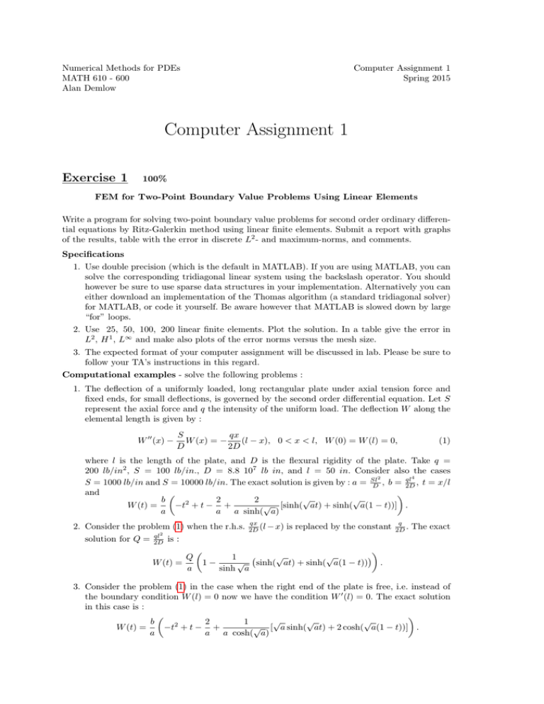
Numerical Methods for PDEs
MATH 610 - 600
Alan Demlow
Computer Assignment 1
Spring 2015
Computer Assignment 1
Exercise 1
100%
FEM for Two-Point Boundary Value Problems Using Linear Elements
Write a program for solving two-point boundary value problems for second order ordinary differential equations by Ritz-Galerkin method using linear finite elements. Submit a report with graphs
of the results, table with the error in discrete L2 - and maximum-norms, and comments.
Specifications
1. Use double precision (which is the default in MATLAB). If you are using MATLAB, you can
solve the corresponding tridiagonal linear system using the backslash operator. You should
however be sure to use sparse data structures in your implementation. Alternatively you can
either download an implementation of the Thomas algorithm (a standard tridiagonal solver)
for MATLAB, or code it yourself. Be aware however that MATLAB is slowed down by large
“for” loops.
2. Use 25, 50, 100, 200 linear finite elements. Plot the solution. In a table give the error in
L2 , H 1 , L∞ and make also plots of the error norms versus the mesh size.
3. The expected format of your computer assignment will be discussed in lab. Please be sure to
follow your TA’s instructions in this regard.
Computational examples - solve the following problems :
1. The deflection of a uniformly loaded, long rectangular plate under axial tension force and
fixed ends, for small deflections, is governed by the second order differential equation. Let S
represent the axial force and q the intensity of the uniform load. The deflection W along the
elemental length is given by :
W 00 (x) −
S
qx
W (x) = −
(l − x), 0 < x < l, W (0) = W (l) = 0,
D
2D
(1)
where l is the length of the plate, and D is the flexural rigidity of the plate. Take q =
200 lb/in2 , S = 100 lb/in., D = 8.8 107 lb in, and l = 50 in. Consider also the cases
2
ql4
S = 1000 lb/in and S = 10000 lb/in. The exact solution is given by : a = Sl
D , b = 2D , t = x/l
and
√
√
2
2
b
√ [sinh( at) + sinh( a(1 − t))] .
−t2 + t − +
W (t) =
a
a a sinh( a)
2. Consider the problem (1) when the r.h.s.
solution for Q =
ql2
2D
qx
2D (l − x)
is replaced by the constant
q
2D .
The exact
is :
W (t) =
Q
a
1−
√
√
1
√ sinh( at) + sinh( a(1 − t)) .
sinh a
3. Consider the problem (1) in the case when the right end of the plate is free, i.e. instead of
the boundary condition W (l) = 0 now we have the condition W 0 (l) = 0. The exact solution
in this case is :
√
√
√
b
2
1
2
√ [ a sinh( at) + 2 cosh( a(1 − t))] .
W (t) =
−t + t − +
a
a a cosh( a)
If the r.h.s.
qx
2D (l−x)
is replaced by the constant
W (t) =
Q
a
1+
q
2D
then the exact solution is (with Q =
ql2
2D )
:
√
√
√
sinh a
√ sinh( at) − cosh( at) .
cosh a
4. A thin rod made of three different materials with insulated lateral surface has ends kept at
temperature 0 and π4 + 32 degrees respectively. The steady state distribution of the temperature
u(x) is a solution to the problem : −(ku0 )0 = 0, x ∈ (0, 1), u(0) = 0, u(1) = π4 + 23 , where
k(x) = 1 for x ∈ (0, π/6) ; k(x) = 2, for x ∈ (π/6, π/4), and k(x) = 3 for x ∈ (π/4, 1). The
6
4
3
exact solution u(x) is a piece-wise linear function defined as 12
π x, π x + 1, and π x + 2 in
the corresponding intervals of definition of k(x).