Supplemental Material for “Can Visual Recognition Benefit from Auxiliary Information in Training?”
advertisement
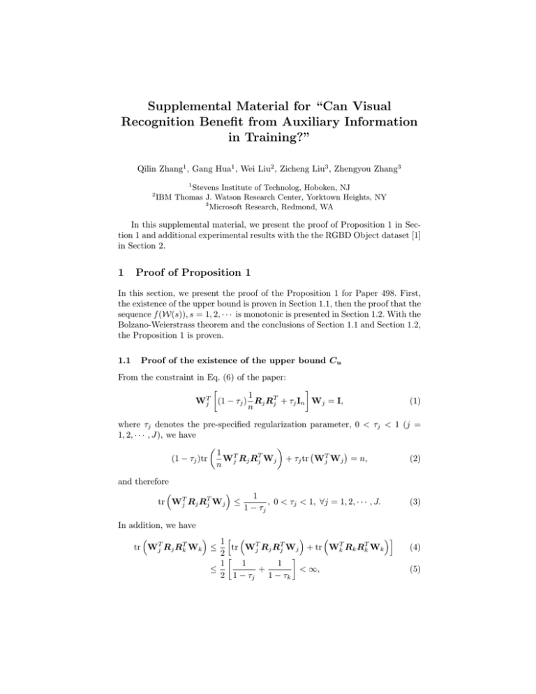
Supplemental Material for “Can Visual Recognition Benefit from Auxiliary Information in Training?” Qilin Zhang1 , Gang Hua1 , Wei Liu2 , Zicheng Liu3 , Zhengyou Zhang3 1 2 Stevens Institute of Technolog, Hoboken, NJ IBM Thomas J. Watson Research Center, Yorktown Heights, NY 3 Microsoft Research, Redmond, WA In this supplemental material, we present the proof of Proposition 1 in Section 1 and additional experimental results with the the RGBD Object dataset [1] in Section 2. 1 Proof of Proposition 1 In this section, we present the proof of the Proposition 1 for Paper 498. First, the existence of the upper bound is proven in Section 1.1, then the proof that the sequence f (W(s)), s = 1, 2, · · · is monotonic is presented in Section 1.2. With the Bolzano-Weierstrass theorem and the conclusions of Section 1.1 and Section 1.2, the Proposition 1 is proven. 1.1 Proof of the existence of the upper bound Cu From the constraint in Eq. (6) of the paper: 1 T T Wj (1 − τj ) Rj Rj + τj In Wj = I, n (1) where τj denotes the pre-specified regularization parameter, 0 < τj < 1 (j = 1, 2, · · · , J), we have 1 T Wj Rj RTj Wj + τj tr WjT Wj = n, (2) (1 − τj )tr n and therefore tr WjT Rj RTj Wj ≤ 1 , 0 < τj < 1, ∀j = 1, 2, · · · , J. 1 − τj In addition, we have 1h i tr WjT Rj RTk Wk ≤ tr WjT Rj RTj Wj + tr WkT Rk RTk Wk 2 1 1 1 + < ∞, ≤ 2 1 − τj 1 − τk (3) (4) (5) 2 Q. Zhang, G. Hua, W. Liu, Z. Liu, Z. Zhang where the inequality (4) follows the property 1 tr(AT A) + tr(BT B) , (6) 2 T which comes from the fact that tr (A − B) (A− B) ≥ 0, because the matrix (A − B)T (A − B) 0. Since tr WjT Rj RTk Wk is bounded, , g(x) = x or x2 , we have 2 1 1 1 < ∞. (7) g tr WjT Rj RTk Wk + ≤ 4 1 − τj 1 − τk tr(BT A) ≤ Considering cjk = 0 or 1, we have J X j6=k 2 J 1 T 1 X 1 1 cjk g tr < ∞, Wj Rj RTk Wk ≤ + n 4n 1 − τj 1 − τk (8) j6=k which shows that the sequence f (W(s)), s = 1, 2, · · · is upper bounded by Cu = 2 J 1 X 1 1 + < ∞. 4n 1 − τj 1 − τk (9) j6=k t u 1.2 Proof that the sequence f (W(s)), s = 1, 2, · · · is monotonically increasing In this section, the monotonic property of the sequence f (W(s)), s = 1, 2, · · · is presented. Following [2–4], we first present a Lemma, and then prove that f (W(s)) ≤ f (W(s + 1)), s = 1, 2, · · · , (10) where s is the iteration index, s = 1, 2, · · · . def Define the function r(Yj , Yk ) = tr( n1 YjT Yk ) = tr( n1 WjT Rj RTk Wk ), therefore, f (W1 (s), · · · , WJ (s)) = J X cjk g[r(Yj (s), Yk (s))]. (11) j,k=1,k6=j Using this notation, we have the following Lemma: Lemma 1. Define def fj (Wj ) = j−1 X J X cjk g r(RTj Wj , Yk (s + 1)) + cjk g r(RTj Wj , Yk (s)) k=1 k=j+1 (12) s.t. WjT Nj Wj = I, Visual Recognition with Auxiliary Information in Training 3 then fj (Wj (s)) ≤ fj (Wj (s + 1)), j = 1, · · · , J. (13) Proof. We prove Lemma 1 in two cases, i.e., g(x) = x2 and g(x) = x. Case 1: when g(x) = x2 , we have fj (Wj ) in the following form, fj (Wj ) = j−1 X J 2 2 X cjk r(RTj Wj , Yk (s + 1)) + cjk r(RTj Wj , Yk (s)) , k=1 k=j+1 (14) which can be written as j−1 1X (s) cjk θjk tr(Wj (s)T Rj Yk (s + 1)) fj (Wj (s)) = n k=1 J 1 X (s) cjk θjk tr(Wj (s)T Rj Yk (s)) (15) n k=j+1 j−1 J X X 1 (s) (s) cjk θjk Yk (s) , = tr Wj (s)T Rj cjk θjk Yk (s + 1) + n + k=1 k=j+1 (16) (s) where θjk are defined as (s) θjk ( r (Yj (s), Yk (s + 1)) if k = 1, · · · , j − 1 = . r (Yj (s), Yk (s)) if k = j + 1, · · · , J Note that in Eq. (16), the term P (s) j−1 k=1 cjk θjk Yk (s + 1) + (17) (s) k=j+1 cjk θjk Yk (s) PJ is equivalent to the definition of Zj (s), hence fj (Wj ) can be simplified as 1 T n tr(Wj Rj Zj (s)). Considering the following optimization problem: 1 maxWj tr(WjT Rj Zj (s)), s.t. WjT Nj Wj = I, n (18) whose solution is exactly † Wj (s + 1) = Nj−1 Rj Zj (s) [Zj (s)T RTj Nj−1 Rj Zj (s)]1/2 , (19) tr(Wj (s)T Rj Zj (s)) ≤ tr(Wj (s + 1)T Rj Zj (s)). (20) we have 4 Q. Zhang, G. Hua, W. Liu, Z. Liu, Z. Zhang Similarly, the following equations can be obtained: fj (Wj (s)) = j−1 X k=1 ≤ j−1 X J X (s) cjk θjk r(Yj (s), Yk (s + 1)) + (s) cjk θjk r(Yj (s), Yk (s)) k=j+1 (s) cjk θjk r(Yj (s + 1), Yk (s + 1)) k=1 J X + (s) cjk θjk r(Yj (s + 1), Yk (s)). (21) k=j+1 Considering that cjk is either 0 or 1, we hence have cjk = c2jk . Applying the Cauchy-Schwartz inequality, we have fj (Wj (s)) ≤ j−1 X (s) c2jk θjk r(Yj (s + 1), Yk (s + 1)) + k=1 J X (s) c2jk θjk r(Yj (s + 1), Yk (s)) k=j+1 v uj−1 J 2 2 X uX (s) (s) cjk θjk + cjk θjk ≤t k=1 k=j+1 v uj−1 J X uX 2 2 cjk (r(Yj (s + 1), Yk (s))) ·t cjk (r(Yj (s + 1), Yk (s + 1))) + k=1 k=j+1 v uj−1 J X uX 2 2 =t cjk (r(Yj (s), Yk (s + 1))) + cjk (r(Yj (s), Yk (s))) k=1 k=j+1 v uj−1 J X uX 2 2 ·t cjk (r(Yj (s + 1), Yk (s + 1))) + cjk (r(Yj (s + 1), Yk (s))) k=1 = q k=j+1 fj (Wj (s)) · q fj (Wj (s + 1)). (22) We immediately have fj (Wj (s)) ≤ fj (Wj (s + 1)). This concludes the case 1 scenario. Case 2: when g(x) = x, we have fj (Wj ) = j−1 X cjk r(RTj Wj , Yk (s + 1)) k=1 + J X cjk r(RTj Wj , Yk (s)). (23) k=j+1 (s) Therefore, we can have exactly the same equation as Eq. (16), except that θjk ≡ 1 for all the cases. The same equation as in Eq. (20) can be obtained, which directly implies that fj (Wj (s)) ≤ fj (Wj (s + 1)). This concludes both the case 2 scenario and the entire proof of Lemma. t u Visual Recognition with Auxiliary Information in Training 5 With the conclusion in Lemma 1, we proceed with the proof that the sequence f (W(s)), s = 1, 2, · · · is monotonically increasing. Consider the following subtraction J X [fj (Wj (s + 1)) − fj (Wj (s))] j=1 = j−1 J X X j=1 k=1 + 1 T T Wj (s + 1) Rj Rk Wk (s + 1) cjk g tr n J J X X j=1 k=j+1 − j−1 J X X j=1 k=1 − j−1 J X X j=1 k=1 = − 1h 2 1 T T Wj (s + 1) Rj Rk Wk (s) cjk g tr n 1 T T Wj (s) Rj Rk Wk (s + 1) cjk g tr n 1 cjk g tr Wj (s + 1)T Rj RTk Wk (s + 1) n J X cjk g tr j,k=1,k6=j J X cjk g tr j,k=1,k6=j 1 Wj (s + 1)T Rj RTk Wk (s + 1) n i 1 Wj (s)T Rj RTk Wk (s) ≥ 0. n (24) The last equation in Eq. (24) follows the Lemma 1. This implies that f (W1 (s), · · · , WJ (s)) ≤ f (W1 (s + 1), · · · , WJ (s + 1)) i.e., f (W(s)) ≤ f (W(s + 1)), s = 1, 2, · · · . (25) (26) Using Eq. (8), Eq. (26), the bounded sequence f (W(s)), s = 1, 2, · · · is monotonically increasing. According to the Bolzano-Weierstrass theorem, the sequence will converge, i.e., Proposition 1 is proven. 2 Additional Experimental Results With the same RGBD Object dataset and experimental settings from [1] and [5], we have also conducted additional experiments with the state-of-the-art HMPbased features [5]. These additional results are summarized in Table 1–2 (too many entries to fit in a single page). As is seen in Table 1–2, the overall recognition accuracy improves significantly across all methods, as compared to the EMK-based features [1]. In a large portion of the categories, perfect recognition is achieved even with the naive baseline 6 Q. Zhang, G. Hua, W. Liu, Z. Liu, Z. Zhang Table 1. Accuracy Table Part 1 for the Multi-View RGBD Object Instance recognition with HMP features, the highest and second highest values are colored red and blue, respectively. The remaining part is in Table 2. Category SVM SVM2K KCCA apple ball banana bell pepper binder bowl calculator camera cap cellphone cereal box coffee mug comb dry battery flashlight food bag food box food can food cup food jar garlic glue stick greens hand towel instant noodles keyboard kleenex lemon light bulb lime marker mushroom notebook onion orange peach pear pitcher plate pliers potato rubber eraser scissors shampoo soda can 87.62 100 73.74 82.07 100 83.08 100 99.17 100 98.43 100 92.88 96.67 86.34 97.34 100 100 98.08 96.32 98.73 90.91 100 76.76 99.63 100 94.55 98.87 45.02 87.67 67.78 100 99.42 100 98.74 72.46 100 90.04 100 99.66 92.58 63.71 69.61 100 99.35 100 93.33 100 77.78 84.06 100 86.54 100 100 100 95.29 100 85.45 97.33 84.14 97.34 100 99.84 93.02 98.90 100 98.40 100 89.73 100 99.51 95.05 97.36 47.41 97.26 62.22 93.93 100 100 94.64 97.58 100 93.24 100 100 89.96 71.81 75.49 100 99.68 100 92.86 100 81.31 78.88 100 86.54 100 100 100 95.81 100 96.90 97.33 85.46 97.87 100 100 94.39 97.06 100 98.40 100 89.19 100 99.76 95.05 97.36 47.41 96.58 61.11 98.26 100 100 95.90 99.03 100 90.75 100 100 90.39 74.13 71.57 100 99.68 99.55 KCCA RGCCA RGCCA RGCCA +L +L +AL 77.14 92.38 87.62 93.33 100 100 100 100 81.31 80.30 75.25 80.30 77.29 73.31 80.88 73.31 100 100 100 100 86.15 87.31 77.69 87.69 99.44 100 100 100 100 99.17 99.17 99.17 100 100 97.08 100 94.76 95.81 98.43 95.81 100 100 100 100 94.43 99.69 91.64 99.69 96.67 98.00 95.33 98.00 76.65 87.67 85.90 88.55 95.21 100 97.34 100 100 100 96.88 100 99.84 100 100 100 81.67 99.18 98.08 99.32 96.32 97.43 97.06 97.43 91.46 100 97.15 100 96.26 95.99 91.98 95.99 100 100 99.68 100 85.41 85.41 81.08 90.27 100 100 99.63 100 99.76 100 100 100 94.55 96.04 94.55 96.53 96.98 98.87 98.87 98.87 45.82 47.81 44.62 47.81 95.21 91.78 89.04 92.47 58.33 62.78 68.33 62.78 96.75 99.57 100 99.78 100 100 99.42 100 100 99.62 100 100 95.90 96.53 99.37 98.74 98.07 96.62 69.57 99.03 100 100 100 100 90.04 91.81 88.61 91.81 100 100 100 100 99.32 95.59 100 99.32 90.39 93.45 92.58 93.45 65.64 65.25 67.57 71.04 69.61 70.59 74.02 70.59 100 100 100 100 98.39 99.68 94.19 99.68 99.10 100 100 100 DCCA 93.33 100 80.30 83.27 100 87.69 100 99.17 100 95.81 100 100 98.00 88.55 100 100 100 99.32 98.53 100 95.99 100 91.35 100 100 96.53 98.87 47.81 92.47 62.22 99.57 100 100 98.74 99.03 100 93.95 100 99.32 93.45 71.43 71.08 100 99.68 100 Visual Recognition with Auxiliary Information in Training 7 Table 2. Continued from Table 1: Accuracy Table Part 2 for the Multi-View RGBD Object Instance recognition with HMP features, the highest and second highest values are colored red and blue, respectively. Category sponge stapler tomato tooth brush tooth paste water bottle average SVM 99.49 80.12 69.69 99.48 100 97.32 92.62 SVM2K 100 73.59 81.59 100 100 95.98 93.35 KCCA KCCA+L RGCCA RGCCA+L RGCCA+AL DCCA 100 99.83 99.83 99.83 99.83 99.83 76.56 76.56 81.90 81.90 82.20 82.49 83.85 83.85 80.45 68.56 80.45 80.45 99.48 96.91 98.97 99.48 98.97 98.97 100 100 100 100 100 100 95.71 94.64 96.25 96.78 96.25 96.25 93.87 91.85 93.93 92.40 94.35 94.62 SVM algorithm, However, the advantage of the proposed method is revealed in some of the challenging categories. Overall, with the HMP-based features, “KCCA+L” and the “RGCCA+L” algorithms cannot match the SVM baseline, and the “SVM2K” and “KCCA” algorithms are only marginally better than the baseline. The “RGCCA” and “RGCCA+AL” algorithms offer some improvements, while the proposed DCCA algorithm achieves the highest overall recognition accuracy. Considering there are more than 13,000 testing samples, the two percent performance improvement means correctly classifying an additional amount of more than 200 samples. References 1. Lai, K., Bo, L., Ren, X., Fox, D.: A large-scale hierarchical multi-view rgb-d object dataset. In: Robotics and Automation (ICRA), 2011 IEEE International Conference on, IEEE (2011) 1817–1824 2. Tenenhaus, A., Tenenhaus, M.: Regularized generalized canonical correlation analysis. Psychometrika 76 (2011) 257–284 3. Tenenhaus, A.: Kernel generalized canonical correlation analysis. Actes des 42è journées de Statistique (2010) 4. Hanafi, M.: Pls path modelling: computation of latent variables with the estimation mode b. Computational Statistics 22 (2007) 275–292 5. Bo, L., Ren, X., Fox, D.: Unsupervised feature learning for rgb-d based object recognition. ISER, June (2012)
