Robust Late Fusion with Rank Minimization
Supplementary Material
Guangnan Ye† , Dong Liu† , I-Hong Jhuo†‡ , Shih-Fu Chang†
†
Dept. of Electrical Engineering, Columbia University
‡
Dept. of Computer Science and Information Engineering, National Taiwan University
{yegn,dongliu,sfchang}@ee.columbia.edu, ihjhuo@gmail.com
Theorem 1. Given a set of n skew-symmetric matrices Ti ,
the SVT solver employed by Algorithm 1 produces a skewsymmetry matrix T̂ if the spectrums between the dominant
singular values are separated.
Since T is skew-symmetric, the decomposed component
Z is also skew-symmetric. Then Z has a block-diagonal
form:


0
λ1
−λ1 0





0
λ2




−λ2 0




.
Z=



.




.



0
λj 
−λj 0
( 0 λ1 )
is
Furthermore, the SVD of the block matrix −λ
1 0
given
by
(
) (
) (
) (
)
0
λ1
0 1
λ1 0
−1 0
=
×
×
.
−λ1 0
1 0
0 λ1
0 1
Proof. Following the proof in [1], to prove the above theorem, we first introduce some properties of skew-symmetric
matrices. Assuming T is a skew-symmetric matrix with the
property T = −T ⊤ , then the eigenvalues of T are pureimaginary and come in complex-conjugate pairs. Moreover,
the rank of T is even [2]. Then the following lemma characterizes the Singular Value Decomposition (SVD) of a skewsymmetric matrix.
Lemma 1. If T is an m × m skew-symmetric matrix with eigenvalues iλ1 , −iλ1 , iλ2 , −iλ2 , . . . , iλj , −iλj
where λp > 0, p = 1, . . . , j, j = ⌊(m/2)⌋, and i denotes the imaginary unit. Then the SVD of T is given by
T = U DV ⊤ where


λ1


λ1




λ
2




λ
2



.
D=




.




.




λj
λj
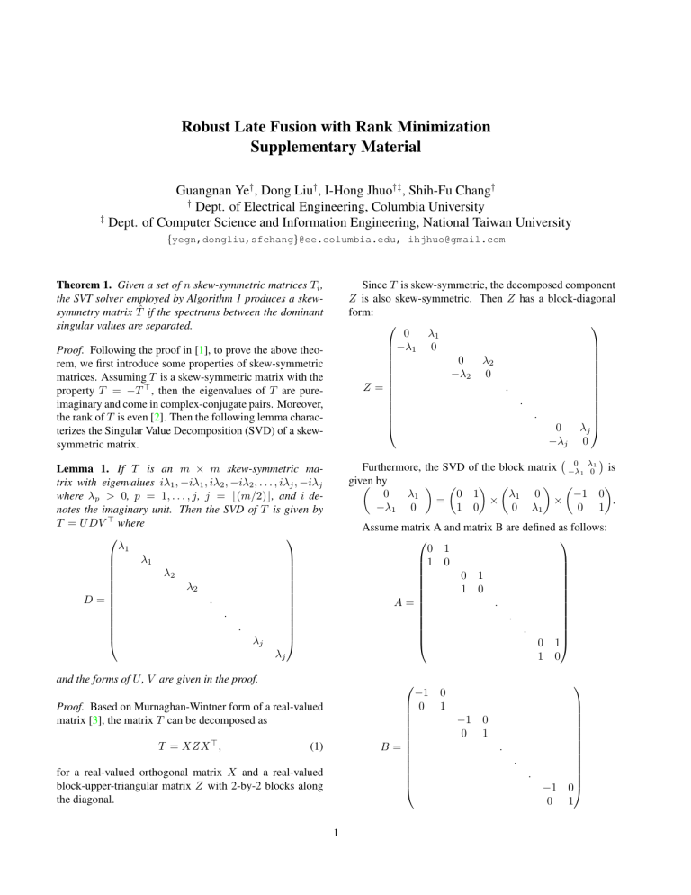
Assume matrix A and matrix B are defined as follows:


0 1
1 0





0 1




1 0




.
A=



.




.



0 1
1 0
and the forms of U , V are given in the proof.

−1 0
0 1


−1 0


0 1

B=






Proof. Based on Murnaghan-Wintner form of a real-valued
matrix [3], the matrix T can be decomposed as
T = XZX ⊤ ,
(1)
for a real-valued orthogonal matrix X and a real-valued
block-upper-triangular matrix Z with 2-by-2 blocks along
the diagonal.
1








.


.


.

−1 0
0 1
Then, the real-valued matrix T has the following decomposition form: T = XADBX ⊤ . We construct U and V
such that U = XA and V ⊤ = BX ⊤ , which are real and
orthogonal. We thus complete the lemma which constructs
the SVD of T .
Next, we use the following lemma to illustrate that
the low rank approximation to a skew-symmetric matrix
T generated by singular value thresholding is also skewsymmetric.
Lemma 2. Let T be an m × m skew-symmetric matrix, and
let λ1 ≥ λ2 ≥ . . . ≥ λj > λj+1 be the magnitudes of
the singular value pairs. (Recall that the previous lemma
showed that the singular values come in pairs, e.g., (iλp ,
−iλp ), p = 1, 2, . . . , j.). Then the low rank approximation
of T generated by singular value thresholding in an orthogonally invariant norm is also skew-symmetric.
Proof. Since the number of singular values of T is even,
and there is a gap between the kth and the (k + 1)th singular value, we can always get the even number of singular
values if we truncate the singular values based on a threshold. Therefore, based on the SVD form from Lemma 1, we
naturally obtain a skew-symmetric matrix.
Finally, we use the above lemma to prove that, given a set
of n skew-symmetric matrices Ti , our ALM-based algorithm preserves a skew-symmetry matrix T̂ (l) in each iteration,
where l denotes the iterative number.
(0)
(0)
Clearly, from Algorithm 1, T̂ (0) , Ei , Yi , i =
1, . . . , n are all skew-symmetric. In step 4 of our algorithm, we compute the SVD of a skew-symmetric matrix
(0)
(0)
1
n
+ n1 Σni=1 Ti − n1 Σni=1 Ei and truncate the sinnµ Σi=1 Yi
gular values below the threshold, then the obtained T̂ (1) is
skew-symmetric based on Lemma 2 and condition of our
(1)
theorem. In step 5, the obtained Ei is skew-symmetric
(0)
due to the fact that Ti +
Yi
µ
− T̂ (1) is skew-symmetric.
(1)
Similarly, in step 6, we can obtain Yi
which is also
skew-symmetric. As the iteration proceeds, we can obtain
(l)
(l)
skew-symmetric matrices T̂ (l) , Ei , Yi in each iteration.
Therefore, we arrive at a skew-symmetric matrix T̂ when
Algorithm 1 converges, which completes the proof.
References
[1] D. F. Gleich and L. H. Lim. Rank aggregation via nuclear
norm minimization. In KDD, 2011. 1
[2] R. A. Horn and C. R. Johnson. Matrix analysis. Cambridge
University Press, 1985. 1
[3] F. D. Murnaghan and A. Wintner. A canonical form for real matrices under orthogonal transformations. Proceedings
of the National Academy of Sciences of the United States of
America, 1931. 1