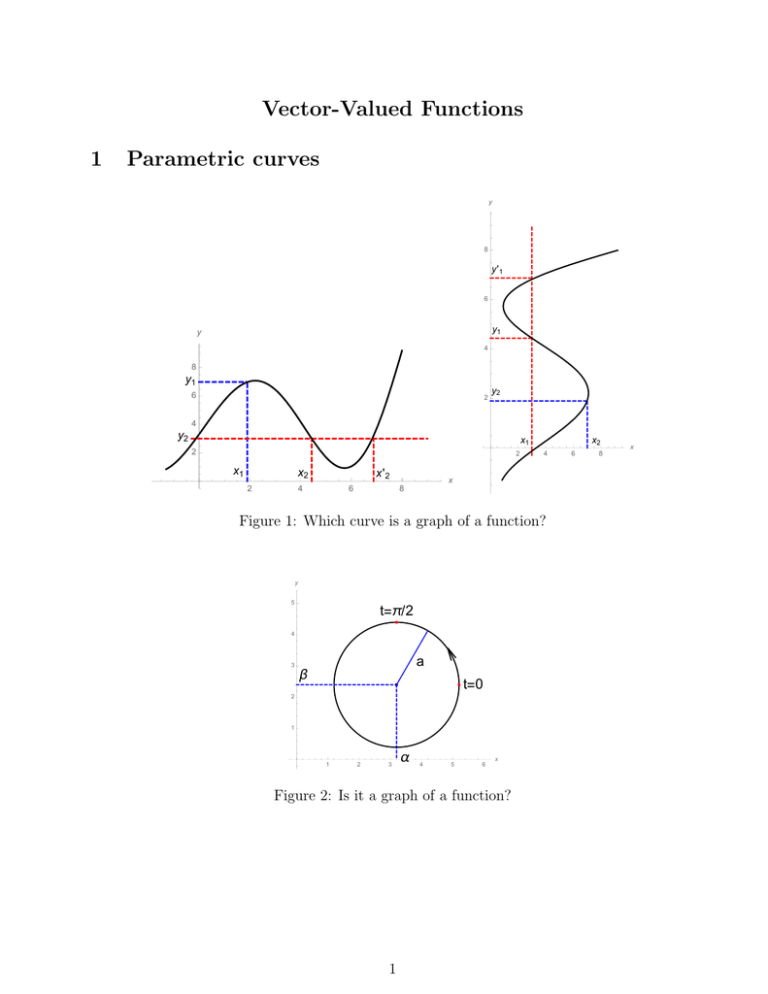
Vector-Valued Functions
1
Parametric curves
y
8
y'1
6
y1
y
4
8
y1
6
2
y2
4
y2
x1
2
2
x1
x2
2
x'2
4
6
x2
4
x
8
Figure 1: Which curve is a graph of a function?
y
5
t=π/2
4
3
a
β
t=0
2
1
1
2
3
α
4
5
6
x
Figure 2: Is it a graph of a function?
1
6
8
x
y
5
t=π/2
4
3
a
β
t=0
2
1
1
2
3
α
4
5
6
x
Figure 3: This curve is not a graph of a function.
This curve is a circle of radius a centred at (α, β)
(x − α)2 + (y − β)2 = a2
It is a parametric curve which can be represented by the eqs
x = α + a cos t ,
y = β + a sin t ,
0 ≤ t ≤ 2π .
In general in 2-space a parametric curve is
x = f (t) ,
y = g(t) ,
t0 ≤ t ≤ t1 .
The graph of a function y = f (x) is a parametric curve
x = t,
y = f (t) .
The graph of a function x = f (y) is a a parametric curve
x = f (t) ,
2
y = t.
z
t=10
t=0
t=100
x
y
t=1
orientation
Figure 4: A parametric curve in 3-space
x = f (t) ,
y = g(t) ,
z = h(t) ,
t0 ≤ t ≤ t1 .
These parametric eqs generate a curve in 3-space called the parametric curve represented
by the eqs, and as t increases the point moves in a specific direction which defines the curve
orientation.
A parametric curve can be considered as a path of a point particle with the parameter t
identified with time.
A parametric curve in n-space is represented by n eqs
x1 = f1 (t) ,
x2 = f2 (t) ,
···
,
3
xn = fn (t) ,
t0 ≤ t ≤ t1 .
Example 1.
(x − α)2 (y − β)2
+
= 1.
a2
b2
y
4
3
y
2.5
2.0
2
1.5
1.0
1
0.5
1
2
3
4
x
0.5
1.0
Figure 5: These are ellipses.
This ellipse can be represented by the eqs
x = α + a cos t ,
y = β + b sin t ,
4
0 ≤ t ≤ 2π .
1.5
2.0
2.5
x
Example 1. Ellipse
(x − α)2 (y − β)2
+
= 1.
a2
b2
Example 2.
(x − α)2 (y − β)2
−
= 1.
a2
b2
(x − α)2 (y − β)2
−
= −1 .
a2
b2
y
y
3
3
2
2
1
1
2
-2
4
6
x
2
-2
4
6
x
Figure 6: These are hyperbolas.
The right (black) branch of the first hyperbola can be represented by the eqs
x = α + a cosh t ,
y = β + b sinh t ,
−∞ < t < ∞ .
because
cosh t =
et + e−t
> 0,
2
sinh t =
et − e−t
,
2
cosh2 t − sinh2 t = 1 .
HW: Find a representation of the left (blue) branch of the first hyperbola, and similar
representations of both branches of the second hyperbola.
5
Example 1. Ellipse
(x − α)2 (y − β)2
+
= 1.
a2
b2
Example 2. Hyperbolas
(x − α)2 (y − β)2
−
= 1.
a2
b2
(x − α)2 (y − β)2
−
= −1 .
a2
b2
Example 3.
y = ax2 .
y 2 = ax .
y
y
2
8
1
6
0.5
4
-1
1.5
x
-1
2
-2
1.0
1
2
x
-2
Figure 7: These are parabolas.
They can be represented by the eqs
x = t,
y = at2 ,
1
x = t2 ,
a
y = t,
Ellipses, hyperbolas and parabolas are conic sections.
6
−∞ < t < ∞ .
Example 4.
x = a cos t ,
y = a sin t ,
z = vt ,
−∞ < t < ∞ .
x = a sin t ,
y = a cos t ,
z = vt ,
−∞ < t < ∞ .
Figure 8: These are circular helixes.
Example 5. Line through ~r0 = (x0 , y0 , z0 ) in the direction of the vector ~v = (vx , vy , vz )
x = x0 + vx t ,
y = y0 + vy t ,
z = z0 + vz t ,
−∞ < t < ∞ .
Example 5b. Find parametric equations for the line through (2, 0, 0) and (0, 4, 3).
���������
Figure 9: This is the line through (2, 0, 0) and (0, 4, 3).
Let t = 0 correspond to (2, 0, 0), and let t = 1 corresponds to (0, 4, 3). Then,
x(1) = x0 + vx = 0
=⇒
vx = −2 ,
y(0) = y0 = 0 ,
y(1) = y0 + vy = 4
=⇒
vy = 4 ,
z(0) = z0 = 0 ,
z(1) = z0 + vz = 3
=⇒
vz = 3 .
x(0) = x0 = 2 ,
Thus
x = 2 − 2t ,
y = 4t ,
z = 3t ,
7
−∞ < t < ∞ .
Example 5. Line through ~r0 = (x0 , y0 , z0 ) in the direction of the vector ~v = (vx , vy , vz )
x = x0 + vx t ,
y = y0 + vy t ,
z = z0 + vz t ,
−∞ < t < ∞ .
Example 6. The same line as in Example 5
1
x = x0 − vx t ,
2
1
y = y0 − vy t ,
2
1
z = z0 − vz t ,
2
−∞ < t < ∞ .
Example 7. The same line as in Examples 5 and 6
1
x = x0 − vx (t − t0 ) ,
2
1
y = y0 − vy (t − t0 ) ,
2
1
z = z0 − vz (t − t0 ) .
2
Example 8. This is a segment of the same line as in Examples 5, 6 and 7
x = x0 + vx t3 ,
y = y0 + vy t3 ,
z = z0 + vz t3 ,
−1 ≤ t ≤ 1 .
Example 9. This is a segment of the same line as in Examples 5, 6 and 7 but it is run twice!
x = x0 + vx (t − 1)2 ,
y = y0 + vy (t − 1)2 ,
z = z0 + vz (t − 1)2 ,
0 ≤ t ≤ 2.
∃ ∞ many parametric eqs representing the same curve.
Make a change t = γ(τ ) where γ(τ ) is a one-to-one function on the interval τ0 ≤ τ ≤ τ1 of
interest.
t
t
t18
1.0
6
0.5
4
-1.0
t0
0.5
-0.5
1.0
τ
-0.5
2
-1.0
-0.5
τ0 0.5
1.0
1.5
2.0
τ12.5
τ
t = τ 3;
Figure 10: γ(τ0 ) = t0 , γ(τ1 ) = t1 ;
The parameterisations are considered as equivalent if γ 0 (τ ) 6= 0 for τ0 ≤ τ ≤ τ1 . If γ 0 (τ ) > 0
the curves have the same orientation.
Example.
x = cos t ,
t = −τ
t=τ−
=⇒
π
2
=⇒
y = sin t ,
x = cos τ ,
x = sin τ ,
8
y = − sin τ ,
y = − cos τ .
2
Vector-Valued Functions
x = f (t), y = g(t), z = h(t)
~r(t) = x(t), y(t), z(t)
z
~r(t) = f (t)~i + g(t)~j + h(t)~k
r(t)
Thus, ~r is a function of t:
~r = ~r(t).
k
i
y
j
x
This is a vector-valued function of a real variable t.
x(t), y(t), z(t) are components of ~r(t).
The graph of ~r(t) is the parametric curve C described by the components of ~r(t).
~r(t) is called the radius vector for the curve C.
The domain of ~r(t) is the intersection of domains of x(t), y(t), z(t).
It is called the natural domain of ~r(t).
Example.
~r(t) =
√
t − 1~i + ln(3 − t)~j +
1 ~
k.
t−2
D(~r) = [1, 2) ∪ (2, 3) .
3
Vector form of a line segment
r0
If ~r0 is a vector with its initial point at O
t(r1 - r0)
then the line through the terminal point
~r0 and parallel to ~v is
r
~r = ~r(t) = ~r0 + t ~v .
r1
So, ~r(0) = ~r0 , ~r(1) = ~r1 = ~r0 + ~v
O
⇒ ~r(t) = ~r0 + t(~r1 − ~r0 ) = (1 − t)~r0 + t ~r1
This is a two-point form of a line.
If 0 ≤ t ≤ 1, then ~r = (1 − t)~r0 + t ~r1 represents the line segment from ~r0 to ~r1 .
9
4
Calculus of Vector-valued Functions
lim ~r(t) =
t→a
lim x(t) ~i + lim y(t) ~j + lim z(t) ~k ,
t→a
t→a
t→a
where all the three limits must exist.
A vector-valued function is continuous at t = a (or on an interval I) if all its components
are. Then
lim ~r(t) = ~r(a) ∀a ∈ I .
t→a
Derivative of ~r with respect to t is the following vector
~r 0 (t) = x0 (t)~i + y 0 (t)~j + z 0 (t)~k .
~r(t) is differentiable if all its components are.
Notations
d
~r(t) ,
dt
d~r
,
dt
~r 0 (t) ,
Derivative Rules
1. dtd a ~r1 (t) + b ~r2 (t) = a ~r1 0 (t) + b ~r2 0 (t) ,
2. dtd f (t) ~r(t) = f 0 (t) ~r(t) + f (t) ~r 0 (t) ,
~r 0 ,
~r˙ (t) ,
~r˙ ,
d
[~r(t)] .
dt
a, b are const
y
y
r(t+ϵ)-r(t)
8
r(t+ϵ)
8
6
r'(t)
6
r(t)
r(t)
→0
−−→
4
4
C
C
2
2
0.2
0.4
0.6
0.8
1.0
x
0.2
0.4
0.6
0.8
1.0
x
If ~r 0 (t) 6= 0 and it is positioned with its initial point at the terminal point of ~r then ~r 0 is
tangent to C and points in the direction of increasing parameter.
In mechanics it is velocity of a particle moving along C.
Example.
√
π
3
~r(t) = 2 cos t~i + 1 + 3e2t ~j +
2
~r 0 (t) =?
10
Z
1
ln t
e3u ~
du k .
u
5
Tangent lines to graphs of vector-valued functions
Let P be a point on the graph
y
8
C of a VV function ~r(t), and let
r ' (t0 )
~r 0 (t0 ) 6= 0 where ~r(t0 ) is the
P
6
radius vector from O to P .
r(t0 )
Then, ~r 0 (t0 ) is a
4
C
tangent vector to C at P ,
2
and the line through P that is
0.2
0.4
0.6
0.8
1.0
parallel to ~r 0 (t0 ) is the tangent
x
line to C at P .
The tangent line is given by the vector eq
~
R(t)
= ~r0 + t ~v0 ,
The unit tangent vector is T~ =
~v
|~v |
=
~v0 = ~r 0 (t0 ) ,
~r0 = ~r(t0 ) .
~
r0
.
|~
r 0|
Example.
~r(t) = a sin t~i + a cos t ~j + v t ~k ,
~r 0 (t) =? ,
6
|~r 0 (t)| =? ,
T~ (t) =? ,
π
~
R(t)
at t = ? ,
3
Derivatives of dot and cross products
y
8
r2
~r1 = (x1 , y1 , z1 ), ~r2 = (x2 , y2 , z2 ) .
6
~r1 · ~r2 = x1 x2 + y1 y2 + z1 z2
r1
= |~r1 | |~r2 | cos α = ~r2 · ~r1
4
α
2
0.2
0.4
0.6
0.8
1.0
x
11
~r1 × ~r2 = +(y1 z2 − y2 z1 )~i
r1 x r2
−(x1 z2 − x2 z1 ) ~j
+(x1 y2 − x2 y1 ) ~k
r2
= α
~i ~j ~k x1 y1 z1 = −~r2 × ~r1
x2 y2 z2 |~r1 × ~r2 | = |~r1 | |~r2 | sin α ,
r1
~r1 × ~r2 ⊥ ~r1 and ~r2 .
d
d~r1
d~r2
(~r1 · ~r2 ) =
· ~r2 + ~r1 ·
,
dt
dt
dt
d~r1
d~r2
d
(~r1 × ~r2 ) =
× ~r2 + ~r1 ×
.
dt
dt
dt
Theorem. If |~r(t)| is a constant then ~r(t) · ~r 0 (t) = 0.
Proof:
d
d
(~r · ~r) = |~r|2 = 0 ,
dt
dt
d
d~r
d~r
d~r
(~r · ~r) =
· ~r + ~r ·
= 2~r ·
,
dt
dt
dt
dt
Thus, ~r(t) ⊥ ~r 0 (t), and T~ (t) ⊥ T~ 0 (t).
Example. A curve on the surface of a sphere that is centred at the origin has |~r(t)|=const,
thus ~r(t) ⊥ ~r 0 (t).
12
7
Integrals of Vector-valued Functions
Z
b
~r(t)dt =
b
Z
a
Z b
Z b
x(t)dt ~i +
y(t)dt ~j +
z(t)dt ~k
a
a
a
Example 1.
Z
1
(
√
3t + 1~i + e2t~j + 3 sin(πt)~k )dt = ?
0
Rules of integration
Z b
Z b
Z b
(c1~r1 (t) + c2~r2 (t))dt = c1
~r1 (t)dt + c2
~r2 (t)dt
a
a
a
~
An antiderivative for a v-v function ~r(t) is a v-v function R(t)
such that
Z
0
~
~ +C
~
R (t) = ~r(t) =⇒
~r(t)dt = R(t)
Example 2.
Z
(
1 ~
i + t cos(t2 − 1)~j )dt = ?
t+1
Integration properties
Z
d
~r(t)dt = ~r(t) and
dt
Z
~
~r 0 (t)dt = ~r(t) + C
Fundamental Theorem of Calculus
Z b
~ b = R(b)
~
~
~r(t)dt = R(t)
− R(a)
a
a
Example 3.
Z
1
(
0
1 ~
i + t cos(t2 − 1)~j )t = ?
t+1
Example 4. Find ~r(t) given that
1
~r 0 (t) = ( t+1
, t cos(t2 − 1) ), ~r(1) = (1, 3)
13
8
Arc Length Parametrisation
We say that ~r(t) is smoothly parameterised or that ~r(t) is a smooth function of t if ~r 0 (t)
is continuous and ~r 0 (t) 6= 0 for any allowed value of t.
Geometrically it implies that the tangent vector ~r 0 (t) varies continuously along the curve.
For this reason a smoothly parameterised function is said to have a continuously turning
tangent vector.
Example 1.
~r(t) = a cos t~i + a sin t ~j + vt ~k ,
~r 0 (t) = ?
Example 2.
~r(t) = t2 ~i + t3 ~j ,
~r 0 (t) = ?
Change of Parameter
y
y
y
3.0
3.0
3.0
2.5
2.5
2.5
r(t)
2.0
s
2.0
r(s)
1.5
1.5
1.5
1.0
1.0
1.0
0.5
0.5
0.5
0.5
1.0
1.5
2.0
2.5
3.0
x
0.5
1.0
1.5
2.0
2.5
r(ϕ)
2.0
3.0
x
0.5
1.0
1.5
2.0
ϕ
2.5
3.0
x
Figure 11: Parameters: time; distance travelled; angle φ
A change of parameter in a v-v function ~r(t) is a substitution
t = g(τ ) that produces a new v-v function ~r(g(τ )) having the same graph as ~r(t).
Example. Find a change of parameter t = g(τ ) for the circle ~r(t) = cos t~i + sin t ~j, 0 ≤ t ≤ 2π
such that the circle is traced (a) counterclockwise; (b) clockwise; as τ increases over the interval
[0, 1].
Chain rule:
d~r
d~r dt
=
,
dτ
dt dτ
t = g(τ ) .
A change of parameter t = g(τ ) in which ~r(g(τ )) is smooth if ~r(t) is smooth is called a
smooth change of parameter.
It requires dt/dτ 6= 0 ∀τ and dt/dτ continuous. If dt/dτ > 0 it is positive change of
parameter, if dt/dτ < 0 it is negative.
14
Arc Length as a Parameter
z
The arc length L of a parametric curve
t=a
x = x(t), y = y(t), z = z(t), a ≤ t ≤ b:
L=
t=b
Rb
r 2
a
dx
dt
+
2
dy
dt
+
2
dz
dt
dt
y
x
In a vector form ~r(t) = x(t)~i + y(t)~j + z(t)~k
d~r
dx
dy
dz
= ~i + ~j + ~k
dt
dt
dt
dt
=⇒
=⇒
Z b d~r L=
dt a
r d~r dx 2 dy 2 dz 2
=
+
+
dt dt
dt
dt
Z b
|~r 0 (t)| dt .
dt =
a
Example.
x = a cos t
y = a sin t
z = vt
0≤t≤π
L =?
The length of arc measured along the curve from some fixed reference point can serve as a
parameter.
s=-2
1. Select an arbitrary point
on the curve C to serve as a
s=-1
- dir
reference point O.
s=0
O
s=1
s=2
+ dir
2. Choose one direction along C to be positive, and the other to be negative.
3. If P is a point on C, let s be the “signed” arc length along C from O to P , where s is
positive/negative if P is in +/- parts of C.
4. x = x(s), y = y(s), z = z(s) is called an arc length parametrisation of the curve. It
depends on the reference point and direction.
Example.
x = a cos t ,
y = a sin t ,
15
0 ≤ t ≤ 2π
Finding arc length parameterisation
y
r(t0 )
8
O
s
6
Z t d~r du
s=
t0 du
r(t)
P
Since
4
C
ds
dt
r
> 0 it is a positive
= d~
dt
change of parameter from t to s.
2
0.2
0.4
0.6
0.8
1.0
x
Example 1.
~r = cos t~i + sin t ~j + t ~k
Example 2. A line through ~r0 and parallel to ~v
Properties of arc length parameterisation
d~r = > 0 (it is speed).
1. ∀t, ds
dt
dt
r ds = =1
2. ∀s, the tangent vector has length 1: d~
ds
ds
d~r 3. If dt = 1 ∀t, then ∀t0 , s = t − t0 is the arc length parameter that as the reference point
at t = t0 .
16