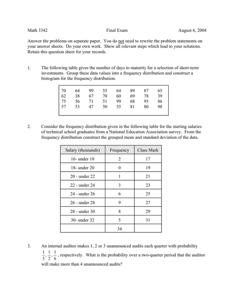
Math 3342
Final Exam
August 6, 2004
Answer the problems on separate paper. You do not need to rewrite the problem statements on
your answer sheets. Do your own work. Show all relevant steps which lead to your solutions.
Retain this question sheet for your records.
1.
The following table gives the number of days to maturity for a selection of short-term
investments. Group these data values into a frequency distribution and construct a
histogram for the frequency distribution.
70
62
75
57
2.
64
38
56
53
99
67
71
47
55
70
51
50
64
60
99
55
89
69
68
81
87
78
95
80
65
39
86
98
Consider the frequency distribution given in the following table for the starting salaries
of technical school graduates from a National Education Association survey. From the
frequency distribution construct the grouped mean and standard deviation of the data.
Salary (thousands)
Frequency
Class Mark
16- under 18
2
17
18- under 20
0
19
20 - under 22
1
21
22 - under 24
3
23
24 - under 26
6
25
26 - under 28
9
27
28 - under 30
8
29
30- under 32
5
31
34
3.
An internal auditor makes 1, 2 or 3 unannounced audits each quarter with probability
1 1 1
, , , respectively. What is the probability over a two-quarter period that the auditor
3 2 6
will make more than 4 unannounced audits?
4.
Let A and B be events for which P(A) = 0.51, P(B) = 0.43 and P( A ∪ B ) = 0.64. Find:
a.
P( A ∩ B )
b.
P( A ∩ B )
c.
P( A ∩ B )
d.
P( A ∪ B )
5.
Studies show that 60% of American families use physical aggression to resolve conflict.
Suppose that 20 families are to be selected at random. Find the probability that more
than half use physical aggression to resolve conflict?
6.
The World Almanc reports that the mean travel time to work in New York is 59 minutes.
Let x be the time, in minutes, that it takes a randomly selected worker to get to work on a
randomly selected day. If the travel times are normally distributed with a standard
deviation of 11 minutes, find P(55 < x < 67).
7.
According to the Daily Racing Form, the probability is about 0.67 that the favorite in a
horse race will finish in the money (first, second or third place). Find the probability that
in the next 200 races the favorite will finish in the money at least 150 times.
8.
The U.S. Bureau of Labor Statistics collects information on the ages of people in the
civilian labor force and publishes the results in Employment and Earnings. The
following table summarizes the ages of 35 randomly selected people in the civilian labor
force. Construct a 90% confidence interval for the mean age, μ , of all people in the
civilian labor force. Assume that the population standard deviation of age is 9.5. (Note:
the sum of the data is 1,262.)
22
33
60
27
42
9.
58
16
41
31
40
40
49
28
33
31
42
29
35
24
34
43
30
37
34
38
32
43
51
28
35
34
37
37
39
29
The Health Insurance Association of America reports in Survey of Hospital Semi-Private
Room Charges that the mean daily charge for a semi-private room in America hospitals
was $253 in 1988. In that same year, a random sample of 30 Massachusetts hospitals
yielded a mean daily semi-private room charge of $260.68 with a standard deviation of
$12.77. Does this data provide sufficient evidence to conclude that for 1988, the mean
daily semi-private room charge in Massachusetts hospitals exceeded the national mean of
$253? (Use a significance level of α = 0.05.)
10.
Surveys are conducted by the Northwestern University Placement Center, Evanston, IL,
on starting salaries for college graduates. Results of the surveys can be found in the
publication The Northwestern Lindquist-Endicott Report. The following table
summarizes for two independent random samples of 32 accounting and 35 liberal arts
graduates their starting annual salaries (in thousands). The data is given in thousands of
dollars and is rounded to the nearest hundred. At the 5% significance level, does it
appear that the accounting graduates have a higher mean starting salary than liberal arts
graduates? Assume that the population standard deviation for starting salaries for
accounting graduates is $1.73 thousand and that for the liberal arts graduates is $1.82
thousand.
Accounting
24.9
23.4
24.0
26.2
25.5
24.9
22.2
21.5
20.4
25.3
22.0
25.9
20.4
25.4
22.1
22.5
23.3
26.8
21.7
24.8
22.4
25.8
21.0
25.4
20.9
22.6
23.0
25.3
24.5
24.2
24.7
26.6
Liberal Arts
20.0
18.7
19.1
20.8
19.9
18.3
20.9
21.4
16.8
23.8
21.1
20.4
19.2
22.7
19.1
16.3
21.3
18.3
19.6
17.1
19.1
20.0
20.8
16.3
20.6 21.0
17.7 18.0
19.0 18.7
19.5
17.2
19.2
20.5
20.5
(Note: The sum of the accounting data is $759.6 thousand and the sum of the liberal arts
data is $682.9 thousand.)
11.
The A.C. Nielsen Company collects data on the TV viewing habits of Americans and
publishes the information in Nielsen Report on Television. The following table presents
for 12 randomly selected married couples their weekly viewing times, in hours. At the
5% significance level, does it appear that married men watch less TV, on the average,
than married women?
Husband
Wife
Husband
Wife
21
56
34
30
41
35
24
55
55
34
31
38
38
27
30
31
30
15
45
29
41
37
35
17
(Note: For d = husband_hours - wife_hours we have ∑ d = -53 and ∑ d = 815.)
2
12.
In planning a new airline route, management assumed that the variance of month
passenger traffic would be 30 (thousands of passengers). The numbers of monthly
passengers (in thousands) during the first 15 months were as follows:
55
54
51
55
49
55
50
56
48
46
54
47
52
48
54
Assuming that the number of passengers is normally distributed, test the hypothesis that
the variance of the monthly passenger traffic is 30 – use an α = 0.05 level of
significance.
13.
It is claimed that 40 percent of all families who own a house in California have an annual
income of $65,000 or more. A random sample of 1100 families who own houses in
California reveals that 455 have an income of $65,000 or more. Construct a 98%
confidence interval for the true proportion of families who own a house in California who
have an annual income of $65,000 or more.
14.
Consider the following table showing a relationship between Annual Income and
Consumption (in thousands).
Observation
i
Income
xi
Consumption
yi
1
$50
$55
2
58
63.5
3
68
65
4
47
52.5
5
53
53
6
56
52
7
62
59
8
55
56
9
60
61
10
50
48
a.
Fit a straight line to the data set by the method of least squares.
b.
Find a 95% confidence interval for the mean annual consumption when the
annual income is $55 (thousands).