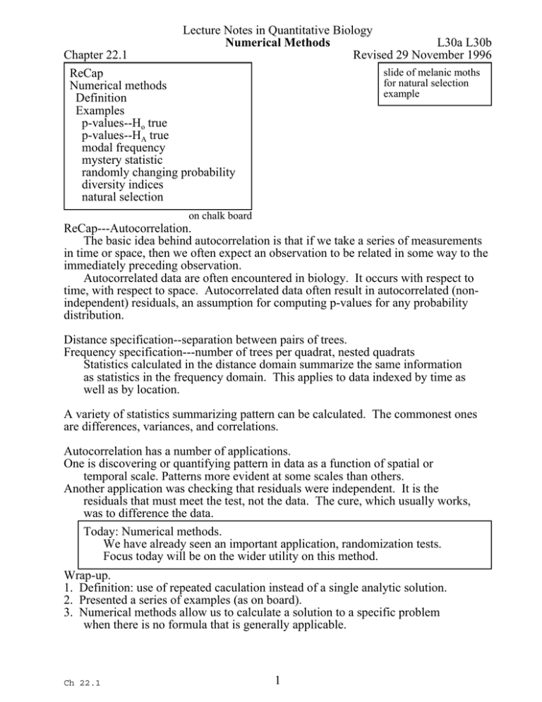
Lecture Notes in Quantitative Biology
Numerical Methods
L30a L30b
Revised 29 November 1996
Chapter 22.1
ReCap
Numerical methods
Definition
Examples
p-values--Ho true
p-values--HA true
modal frequency
mystery statistic
randomly changing probability
diversity indices
natural selection
slide of melanic moths
for natural selection
example
on chalk board
ReCap---Autocorrelation.
The basic idea behind autocorrelation is that if we take a series of measurements
in time or space, then we often expect an observation to be related in some way to the
immediately preceding observation.
Autocorrelated data are often encountered in biology. It occurs with respect to
time, with respect to space. Autocorrelated data often result in autocorrelated (nonindependent) residuals, an assumption for computing p-values for any probability
distribution.
Distance specification--separation between pairs of trees.
Frequency specification---number of trees per quadrat, nested quadrats
Statistics calculated in the distance domain summarize the same information
as statistics in the frequency domain. This applies to data indexed by time as
well as by location.
A variety of statistics summarizing pattern can be calculated. The commonest ones
are differences, variances, and correlations.
Autocorrelation has a number of applications.
One is discovering or quantifying pattern in data as a function of spatial or
temporal scale. Patterns more evident at some scales than others.
Another application was checking that residuals were independent. It is the
residuals that must meet the test, not the data. The cure, which usually works,
was to difference the data.
Today: Numerical methods.
We have already seen an important application, randomization tests.
Focus today will be on the wider utility on this method.
Wrap-up.
1. Definition: use of repeated caculation instead of a single analytic solution.
2. Presented a series of examples (as on board).
3. Numerical methods allow us to calculate a solution to a specific problem
when there is no formula that is generally applicable.
Ch 22.1
1
Definition: Numerical methods substitute repeated calculations for a single analytic
solution. The are used with increasing frequency, as the price of computing power
drops, and the accessibility increases.
Example. p-values Ho true
The first example, by now familiar to us, is the use of "Monte Carlo"
methods to calculate p-values.
Ie to calculate the frequency (probability) of all outcomes more extreme than a
particular observed outcome.
We have a statistic measuring some pattern or some outcome from say an experiment.
We wish to know whether this could have arisen by chance. We need to know the
probability distribution of the statistic, due to chance.
One solution is to assume that the
probability fits one of the standard
statistical frequency distributions:
normal
t
F
Chi-square
Then calculate the p-value (chance of a
more extreme value) from the cumulative
distribution function cdf. This is the
analytic solution. It is based on
mathematical proof.
Use this as opportunity for quick run thru concept of
p-value from pdf and cdf.
Draw pdf for X 2 then translate to cdf,
Write
Ho true
in the distribution.
Run arrows up from statistic X 2 to cdf then across to
probability.
Fig = L30a
Another solution is to use a non-normal error structure (poisson, gamma, binomial,
etc) within the framework of the generalized linear model.
Yet another solution, if we cannot find an appropriate distribution, is to compute our
own distribution of the statistic, from the data at hand. That is, we make the Ho true
by randomizing the data, calculate the statistic, do this repeatedly, until we have a
distribution to compute our p-value. This is a numerical solution. It has neither the
generality nor elegance of a proof. It only works for the case at hand, which is usually
all we need.
Ch 22.1
2
Example -- modal value of the normal distribution
The equation for the normal distribution of
outcomes is:
pdf(x) = xo exp(-(x-:)/F)2
We can use this to calculate frequency of
observations at any value x
At what value x does the normal
distribution pdf(x) have a maximum ?
If we look at the graph, it looks like the
answer is that pdf(x) reaches its maximum
when : = 0 and F = 1.
Chance to review quickly the normal
distribution, centred on zero.
Fig = L30b
Review also notation
E(RF(X) = pdf(X)
For a mathematician, the solution is of course to differentiate,
set the derivative F'(x) equal to zero,
and solve for x when the slope of the function itself is zero.
Suppose were knew nothing about differentiation.
With a little search, and the aid of a programmable calculator we can carry out a
search for the right value.
Search Table:
x
10
5
!5
0
5
0.1
0.001
________________________________________________________________
pdf(x)
10-44
10-11
10-11
1
10-11
.99005 .9999990
Search strategy was to start with a wild guess
at x = 10,
then take a guess downward x = 5,
then a guess further downward at x = !5,
then a point in the middle x = 0,
then another guess in the middle x = 2.5,
then an educated guess close to zero 0.1
then another educated guess close to zero 0.001.
Ch 22.1
3
point at 10 on x axis
beneath normal distribution
Mark each guess on the xaxis below normal curve.
Fill in the search table as
each guess is made.
Example modal value of a distribution (continued)
Using numerical methods to search for location of the maximum value of the normal
distribution. Iterative search shows that the closer to zero, the bigger the value of
pdf(x).
So the maximum value of pdf(x) occurs at pdf(0) ie at :
This illustrates the use of numerical methods rather than analytic methods. Of course
we would use analytic methods for this problem, by differentiating and solving for x.
But in some cases analytic solutions cannot be obtained. Then numerical solutions
are required. For example, Newton's laws of motion are used to compute weather
change, but these are numerical solutions on large computers because the equations
cannot be solved analytically.
Example What is value of the mystery statistic ?
Let Yi = 8 6 9 8 7 9 2 3 4
E(Yi - ST)2 = Dev2 What is the value of the mystery statistic ST that
minimizes the squared deviations from ST ?
What is the value of ST such that Dev2 has the minimum possible value ?
Again, this can be solved analytically. In this case a little more difficult to set the
problem up, but it can be solved by setting up a function, taking the first derivative,
setting equal to zero,
and solving for a.
We can also approach the problem with direct computations. We write out a search
Table of Dev2 as a function of ST, start with wild guesses for ST,
move on to educated guesses, then finally make refined guesses as we home in on the
value of ST that minimizes Dev2.
If we carry this through by searching in this manner, we find that Dev2 reaches its
minimum values when ST = mean(Y)
Ch 22.1
4
Example. Randomly changing probabilities
For standard statistical analyses we often have some theoretical distribution such as F,
or t (a special case or F), or chisquare, or binomial, or normal. This is a theoretical
function that gives us the precise value of the frequency of an outcome of a particular
value x. For example if we have 7 successes out of ten trials we can use the binomial
distribution to calculate the probability of obtaining this result if we had a 50:50
chance of success on each trial. The answer is p = 0.0547, which we know how to
calculate in a spreadsheet or statistical package.
MTB > cdf 7;
SUBC> binomial n=10 p = .5 .
This is an analytic solution. We can also use the analytical solution (the binomial
distribution) if we know that we have a 30% chance of success on each trial.
MTB > cdf 7;
SUBC> binomial n=10 p=.3.
Success is more elusive and so the probability of 7 success is much smaller.
p = 0.0016
What if we had a situation where we knew that the chance of success changes from
trial to trial? We cannot handle this with the binomial distribution, which has a
parameter held constant, such as 50:50 in the first case, or 30:70 in the second.
The analytic solution is to write an equation stating how this parameter changes from
trial to trial, then solve for the distribtuion, then use this analytical solution to
calculate p-values. This is difficult. It was the stuff of Ph.D. theses in statistics in the
1950s.
The numerical solution to the problem is to carry out repeated applications of the
binomial distribution for each trial, each with different parameter (obtained from
random numbers between 0 and 1). Then keep of running tally of the number (or
frequency) of success for 1 trial, 2 trials .... 10 trials. This produces an empirical
distribution of outcomes, from which we can construct a cumulative distribution.
If time allows, review how to construct
cumulative distribution.
Ch 22.1
5
Example Diversity index.
A new example (grad project, Quentin Baldwin, in Winter 1995)
Rarefaction formula for number of species.
Can use numerical methods instead.
No formula for effect on diversity index H = G pi ln pi
where p = proportion of species i in collection of size N
So use numerical methods to investigate this.
Ch 22.1
6
Example Natural Selection.
This material can also be used for last quiz, see Lastquiz.w13 WP file.
This quiz is example of problem solving, in format that is relatively
easy to mark, and so makes good final exam question. The quiz can be
given in the final days, then marked in class, as a form of review.
People do not like to mark other quizzes, so it is best to have each
person mark their own quiz, which they can retain for review.
Here is another example of substituting calculation for analytical solution.
Taken from R. Dawkins The Blind Watchmaker
Picture of melanistic moth on screen, if possible. With brief recap of
selection for dark coloration due to soot on trees in England,
beginning with the industrial revolution.
We are confronted with skilfully designed artifact, such as a watch lying out on the
moor. We say then that this artifact is so improbable that it must have been fabricated
by some watchmaker. We then look at the exquisite design of an organism and
reasoning similarly, ask the nature of the watchmaker. Can natural selection, acting
blindly, be the watchmaker ?
The complexity of the end result would seem to argue against there being a blind
watchmaker. Natural selection is blind, and so couldn't make such an exquisitely
designed watch.
This turns out be be true if we try to assemble the artifact all at once, rather than from
completed subunits.
To show how effective cumulative natural selection can be we will construct a
sentence by natural selection.
"Methinks it is like a weasel"
What is chance of this ? there are 28 places to fill, with 26 letters or blanks.
Construction by chance is 1 in 27 to the 28th power.
Chance of this sentence being constructed by single step selection is 1 in 1040 or so.
Very improbable.
Let's calculate outcomes using "cumulative selection"
Start with 28 random letters
Replicate the sentence with certain chance of mistakes (typically 1 in 106)
Select copy closest to pattern sentence.
Using this selected copy, repeat the process.
Ch 22.1
7
Example Natural Selection. (continued)
How many steps to get perfect adaptation ? (Ie to get the target sentence)
Dawkins wrote a program to do this 1 run
43 steps
next run
64 steps
next run
41 steps
Rather less than 1040 steps.
This is an example of solution by numerical rather than analytical methods. Dawkins
used a series of computations according to his concept of sequential selection to
arrive at an answer. The answer was "around 50 rather than 1040"
The answer was not obtained from an equation.
Dawkins goes on to more complex set-up of the problem in which computer grows
"trees" (organisms) according to certain recursive rules (genes). Results are counterintuitive. The trees were far more complex than one would expect, just using random
mutation + selection relative to template of the environment.
When analytic solutions fail due to complexity of the problem, then numerical
methods become necessary.
Numerical methods produce answers when analytic solution fail.
The bonus in using these quantitative methods is that they will often serve to sharpen
our thinking, as they force us to state the problem in some exact fashion, exact
enough to make calculations.
Ch 22.1
8
Wrap-up.
Examples:
Monte Carlo estimates of p-values
Finding an optimum (maximum) value
E.g. "mystery statistic" (the mean, minimizes squared deviations)
E.g. Finding "best" cladistic tree
Computing fluid flows, using Newton's laws
Computing genetic combinations
Rate of evolution by assembly of subunits
there are many good recipes in quantitative biology, based on analytic formula. Best
to use these when available. but if none are available, computation methods can be
used.
These allow us to calculate a solution in a specific case, when there is no formula that
is generally applicable.
Ch 22.1
9