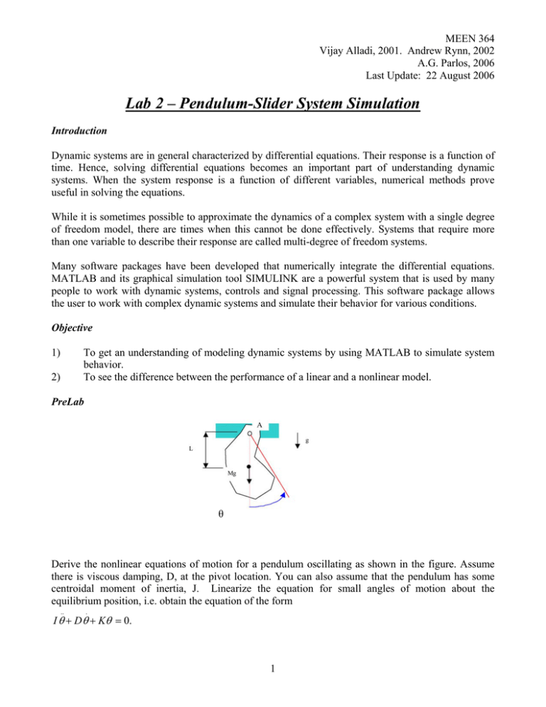
MEEN 364
Vijay Alladi, 2001. Andrew Rynn, 2002
A.G. Parlos, 2006
Last Update: 22 August 2006
Lab 2 – Pendulum-Slider System Simulation
Introduction
Dynamic systems are in general characterized by differential equations. Their response is a function of
time. Hence, solving differential equations becomes an important part of understanding dynamic
systems. When the system response is a function of different variables, numerical methods prove
useful in solving the equations.
While it is sometimes possible to approximate the dynamics of a complex system with a single degree
of freedom model, there are times when this cannot be done effectively. Systems that require more
than one variable to describe their response are called multi-degree of freedom systems.
Many software packages have been developed that numerically integrate the differential equations.
MATLAB and its graphical simulation tool SIMULINK are a powerful system that is used by many
people to work with dynamic systems, controls and signal processing. This software package allows
the user to work with complex dynamic systems and simulate their behavior for various conditions.
Objective
1)
To get an understanding of modeling dynamic systems by using MATLAB to simulate system
behavior.
To see the difference between the performance of a linear and a nonlinear model.
2)
PreLab
θ
Derive the nonlinear equations of motion for a pendulum oscillating as shown in the figure. Assume
there is viscous damping, D, at the pivot location. You can also assume that the pendulum has some
centroidal moment of inertia, J. Linearize the equation for small angles of motion about the
equilibrium position, i.e. obtain the equation of the form
..
.
I θ + D θ + Kθ = 0.
1
MEEN 364
Vijay Alladi, 2001. Andrew Rynn, 2002
A.G. Parlos, 2006
Last Update: 22 August 2006
Lab
The system shown below consists of a pendulum mounted on a slider. It is a two-degree of freedom
system. This is different from the pendulum in the prelab in the sense that the pivot, P, can also move
in a linear fashion.
A
B
O
O'
P
y
C
x
Figure 4-1 - Pendulum-Slider System (drawn by Christopher Cullum)
Theory and analysis of the system
The following free body diagrams will be useful in the analysis of the coupled pendulum system.
Fy
M0
P
Fx
lcg
θ
C
m 1g
Figure 4-2 - Free Body Diagram of Pendulum (drawn by Christopher Cullum)
2
MEEN 364
Vijay Alladi, 2001. Andrew Rynn, 2002
A.G. Parlos, 2006
Last Update: 22 August 2006
Fy
b
F s1
Fx
F s2
M0
F fr
d
m 2g
N
Figure 4-3 - Free Body Diagram of Slider (drawn by Christopher Cullum)
Considering the free body diagrams shown above, we now come up with equations of motion of the
system. First, we go through the kinematics of the different bodies to evaluate the velocities and
accelerations of center of masses. We then use Newton’s laws to come up with the kinetics of the
bodies using the derived velocities and accelerations.
Kinematics:
For the pendulum
r
rc = ( x + b + l sin(θ ))i − l cos(θ ) j
(1)
.
.
.
r
Vc = ( x + l cos(θ ) θ )i + l sin(θ ) θ j
(2)
..
..
. 2
. 2
..
r
ac = ( x + l cos(θ )θ − l sin(θ )θ )i + (l cos(θ )θ + l sin(θ )θ ) j
(3)
This gives
..
..
. 2
r
a x = ( x + l cos(θ ) θ − l sin(θ ) θ )
(4)
. 2
..
r
a y = (l cos(θ ) θ + l sin(θ ) θ )
(5)
For the slider
r
rp = ( x + b )i
(6)
.
r
Vp = x i
(7)
..
r
ap = xi
(8)
Kinetics and the equations of motion from the FBD’s
For the pendulum,
..
..
. 2
Fx = m1 a x = m1 ( x + l cos(θ )θ − l sin(θ )θ )
3
(9)
MEEN 364
Vijay Alladi, 2001. Andrew Rynn, 2002
A.G. Parlos, 2006
Last Update: 22 August 2006
. 2
..
Fy − m1 g = m1 a y = m1 (l cos(θ )θ + l sin(θ )θ )
(10)
..
M 0 − Fx l cos(θ ) − Fy l sin(θ ) = I c θ
(11)
For the slider,
..
− Fs1 − Fs 2 − Fx − F fr = m2 x
(12)
− Fy − m 2 g + N = m 2 ( 0 )
N (d ) − M 0 = 0
(13)
(14)
Assuming both the springs to be identical
Fs1 = Fs 2 = k (Δx)
(15)
Δx = x − l 0 ,
(16)
where
l 0 = un-stretched length of the spring
and
(17)
F fr = μ N
Note: Equation (17) only represents the magnitude of the friction force. A better approximation is
given by the following expression:
F fr = μ ⋅ N ⋅ sign( x& )
But this expression is not used in the present model due to mathematical complications arising when
the sign function is included in the matrix.
Using (9) and (10) in (11) we get
..
..
..
M 0 − m1l ( x cos(θ ) + l θ ) − m1 gl sin(θ ) = I c θ
(18)
From (9), (12), (15) and (17)
..
. 2
..
..
− 2 kΔx − m1 ( x + l (cos(θ ) θ − sin(θ ) θ )) − μ N = m 2 x
(19)
From (10), (13)
. 2
..
N = Fy + m2 g = m1 (l cos(θ )θ + l sin(θ )θ ) + (m1 + m2 ) g
(20)
The above equations will lead to
..
. 2
..
(m1 + m2 ) x + m1l (cos(θ ) + μ sin(θ ))θ + m1l ( μ cos(θ ) − sin(θ ))θ + μ (m1 + m2 ) g + 2kΔx = 0 (21)
..
(22)
..
m1l cos(θ ) x + ( I c + m1l 2 ) θ + m1 gl sin(θ ) = M 0
4
MEEN 364
Vijay Alladi, 2001. Andrew Rynn, 2002
A.G. Parlos, 2006
Last Update: 22 August 2006
Clearly we can see the nonlinearity in the system. Let us rewrite the derivation of the nonlinear model
in a form that is suitable for us to simulate the system.
Lets define the states of the system as below
X1 = x
.
X2 = x
X3 =θ
.
X4 =θ
This gives
.
X1 = X2
(23)
.
X 3 = X4
Using (21), (22), (23) and putting in the form MX& = F , we arrive at the following representation
0
⎡1
⎢0
m1 + m 2
⎢
⎢0
0
⎢
⎣0 m1 l cos( X 3 )
0
0
1
0
0
m1 l(cos( X 3 ) + μ sin( X 3
0
I c + m1 l 2
⎡ . ⎤
X2
⎤⎢ X 1 ⎥ ⎡
⎤
.
⎥
⎢
2
⎢
⎥
))⎥ X 2
− m1 l [ μ cos( X 3 ) − sin( X 3 )] X 4 − μ ( m1 + m 2 ) g − 2 kX 1 ⎥⎥
⎢
⎢
⎥=
⎥⎢ . ⎥ ⎢
⎥
X4
X
3
⎥⎢ . ⎥ ⎢
⎥
M 0 − m 1 gl sin( X 3 )
⎦⎢ X 4 ⎥ ⎣
⎦
⎣
⎦
(24)
This is the nonlinear state space representation of the coupled pendulum system. Both the LHS and
RHS have nonlinearities. Let us also derive the linearized system from the above nonlinear equations.
For this first we need to find out the equilibrium position(s) and apply Taylor’s theorem.
Equilibrium position:
The above equation is of the form
MX& = F .
Equilibrium position is given by
(25)
.
X = 0;
(26)
⇒ X 2 = 0; X 4 = 0; sin( X 3 ) = M 0 / m1 gl; Δx = −
μ (m1 + m2 ) g
,
2k
Since we have used the assumption of viscous damping at the pivot P,
M 0 = −cω = −cX 4
c
X4
is the viscous damping coefficient
is the angular velocity (by definition)
5
(27)
where
MEEN 364
Vijay Alladi, 2001. Andrew Rynn, 2002
A.G. Parlos, 2006
Last Update: 22 August 2006
Since the equilibrium value of X 4 is zero, the equilibrium value of X 3 is given by
sin( X 3 ) = M 0 / m1 gl = 0
and that of X 1 is given by equation (25).
Linearization
Rewriting (25) we have
.
X = M −1 F = g ( X )
(28)
Applying the Taylor series expansion, we have
∂g ( X )
g( X ) = g( X ) X =X +
ΔX
0
∂X X = X 0
(29)
where ΔX represents the perturbation about the equilibrium position X 0 .
.
g ( X ) X = X = 0 since at equilibrium X = 0
by definition
0
∂g ( X )
∂X
=
X =X0
∂( M −1 F )
∂X
=(
X =X0
∂M −1
)F
∂X
+ ( M −1
X =X0
∂F
)
∂X X = X 0
(30)
(31)
Remembering that F ( X 0 ) = 0 , the first term in the above equation vanishes and we arrive at
∂g ( X )
∂X
= ( M −1
X =X0
∂F
)
∂X X = X 0
(32)
Using the values of X 0 we got above , we evaluate
M
X0
0
⎡1
⎢0 m + m
1
2
=⎢
⎢0
0
⎢
m1l
⎣0
⎤
0
m1l ⎥⎥
⎥
1
0
⎥
0 I c + m1l 2 ⎦
0
0
(33)
∂F ⎡ ∂F ∂F ∂F
∂F ⎤
.......
=⎢
⎥
∂X ⎣ ∂X 1 ∂X 2 ∂X 3
∂X n ⎦
(34)
6
MEEN 364
Vijay Alladi, 2001. Andrew Rynn, 2002
A.G. Parlos, 2006
Last Update: 22 August 2006
⎡ 0 ⎤
⎢− 2k ⎥
∂F
⎥
= ⎢
⎢
0 ⎥
∂X 1
⎥
⎢
⎣ 0 ⎦
0
⎤
⎡
⎢m l[cos( X ) + μ sin( X )] X 2 ⎥
∂F ⎢ 1
3
3
4 ⎥
=
⎥
0
∂X 3 ⎢
⎥
⎢
− m1 gl cos( X 3 )
⎦
⎣
⎡1 ⎤
⎢0 ⎥
∂F
=⎢ ⎥
∂X 2 ⎢0⎥
⎢ ⎥
⎣0 ⎦
0
⎡
⎤
⎢− 2m l[ μ cos( X ) − sin( X )] X ⎥
∂F ⎢
1
3
3
4⎥
=
⎥
1
∂X 4 ⎢
⎢
⎥
−c
⎣
⎦
(35)
Evaluating each of the above at the equilibrium position, we get
∂F
∂X
X =X0
⎡ 0
⎢ − 2k
=⎢
⎢ 0
⎢
⎣ 0
1
0
0
0
0
0
0 − m1 gl
0⎤
0 ⎥⎥
= A1
1⎥
⎥
− c⎦
(36)
using ( 29), (30) and (32), gives us the final linearized form of the model written in standard state
space form as
.
(
)
(
where M
X0
−1
X0
)
−1
X = M
A1ΔX
(37)
and A1 can be obtained from (33) and (36) respectively.
Using the fact that
.
.
Δ X = X we finally get
.
(
ΔX = M
)
−1
X0
A1ΔX = A2 ΔX
(38)
This is of the form of the linearized state space.
Writing the linearized state space in the same form as the nonlinear state space ( MX& = F ) yields:
0
⎡1
⎢0 m + m
1
2
⎢
⎢0
0
⎢
m1l
⎣0
0
0
1
0
.
X2
⎤⎡ X 1 ⎤ ⎡
⎤
⎢. ⎥ ⎢
⎥
⎥
− 2 kX 1
m1l ⎥ ⎢ X 2 ⎥ ⎢
⎥
=
.
⎥⎢ X 3 ⎥ ⎢
⎥
0
X4
⎢ ⎥ ⎢
⎥
2⎥ .
I c + m1l ⎦ ⎢ X 4 ⎥ ⎣ − cX 4 − m1 glX 3 ⎦
⎣ ⎦
0
(39)
7
MEEN 364
Vijay Alladi, 2001. Andrew Rynn, 2002
A.G. Parlos, 2006
Last Update: 22 August 2006
Simulations to be run
1) Assume M0 to be viscous drag. The TA will provide you with the different values of the
parameters. You have already had a tutorial on Matlab for solving differential equations of the
.
form M ( x, t ) X = f ( X ) . Run the simulation for initial conditions specified by your TA.
2) Simulate the linear system for the same initial conditions as the nonlinear system.
Issues to be addressed in the report
The lab report should include the plots from all the simulations you have run.
1)
2)
Are the responses of the linear and nonlinear systems the same? For what ranges of operation
is the linearized model a good approximation of the nonlinear one?
Explain the difference between the nonlinear and linear model by looking at the equations and
also the results of simulation.
Things you have learned from this lab
•
•
How to solve differential equations using Matlab.
Differences in performance between nonlinear and linear models.
8