Version date: November 14, 2002
TEACHING NOTE 96-02:
RISK NEUTRAL PRICING IN DISCRETE TIME
C:\CLASSES\TEACHING NOTES\TN96-02.DOC
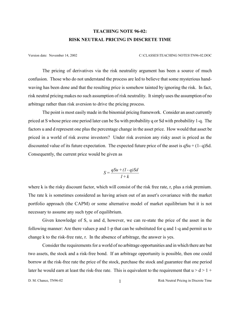
The pricing of derivatives via the risk neutrality argument has been a source of much confusion. Those who do not understand the process are led to believe that some mysterious handwaving has been done and that the resulting price is somehow tainted by ignoring the risk. In fact, risk neutral pricing makes no such assumption of risk neutrality. It simply uses the assumption of no arbitrage rather than risk aversion to drive the pricing process.
The point is most easily made in the binomial pricing framework. Consider an asset currently priced at S whose price one period later can be Su with probability q or Sd with probability 1-q. The factors u and d represent one plus the percentage change in the asset price. How would that asset be priced in a world of risk averse investors? Under risk aversion any risky asset is priced as the discounted value of its future expectation. The expected future price of the asset is qSu + (1- q)Sd.
Consequently, the current price would be given as
S = qSu + (1
1 + k
q)Sd where k is the risky discount factor, which will consist of the risk free rate, r, plus a risk premium.
The rate k is sometimes considered as having arisen out of an asset = s covariance with the market portfolio approach (the CAPM) or some alternative model of market equilibrium but it is not necessary to assume any such type of equilibrium.
Given knowledge of S, u and d, however, we can re-state the price of the asset in the following manner: Are there values p and 1-p that can be substituted for q and 1-q and permit us to change k to the risk-free rate, r. In the absence of arbitrage, the answer is yes.
Consider the requirements for a world of no arbitrage opportunities and in which there are but two assets, the stock and a risk-free bond. If an arbitrage opportunity is possible, then one could borrow at the risk-free rate the price of the stock, purchase the stock and guarantee that one period later he would earn at least the risk-free rate. This is equivalent to the requirement that u > d > 1 +
D. M. Chance, TN96-02 1 Risk Neutral Pricing in Discrete Time

r.
1 The factor u is greater than d by definition. The question is whether d is greater than 1+r. If that is the case, then such an arbitrage is possible. This is certainly an unreasonable possibility for if it existed, everyone would take advantage of it. The interest rate would then have to adjust such that the condition u > 1+r > d. Naturally we could also not have 1+r > u for then it would be possible to short the stock and use the proceeds to buy the bond, assuring ourselves that at worst our return would be 1+r - u. In either case, d > 1+r or 1+r > u, we could guarantee a non-negative payoff without investing any of our own money. Consequently, no arbitrage requires that u > 1 + r > d.
Given that u > 1+r > d, it is possible to find weights p and 1-p that are consistent with the statement pu + (1-p)d = 1+r or the equivalent statement, p = (1+r-d)/(u-d). Since this condition holds, we are permitted to write the stock price as the following:
S = pSu + (1
1 + r
p)Sd
The proof is simple. Divide the expression above by S and multiply by 1 + r giving 1 + r = pu + (1p)d. This is easily converted into p = (1+r-d)/(u-d).
We see from the above equation that the price of an asset can be re-stated simply by changing the probabilities and discounting at the risk-free rate. The only information we are required to know is the volatility (as represented by u and d) and the risk-free rate. We are making no assumptions about how investors feel about risk. Indeed what we have done is perfectly compatible with risk aversion. If by chance investors were risk averse, the above expression gives precisely the value of the asset.
What we have just seen is called the arbitrage theorem . It simply states that if there are no opportunities for arbitrage, then it is possible to state the price of the asset in terms of risk-neutral probabilities where the discounting is done at the risk-free rate. The theorem goes two-ways. If it is possible to state the price of the asset in the above manner, then there are no arbitrage possibilities.
1 The reason we see a A 1" in front of the r and not in front of the u and d is that u and d are already specified as 1 plus the up and down returns. In some writings, r is already specified as 1 plus the risk-free rate.
D. M. Chance, TN96-02 2 Risk Neutral Pricing in Discrete Time

Calling p and 1-p risk neutral probabilities is, however, a source of much confusion.
Alternatively, these probabilities are sometimes called equivalent martingale probabilities . A martingale is a stochastic process in which the expected return of the asset is the current value of the asset. Under the equivalent martingale approach, however, the asset price is re-stated so as to be already discounted at the risk-free rate. In other words, the S is the expectation of the future price already discounted.
There is a definite relationship between the binomial probability and the actual probability.
Define the stock = s risk premium as φ = (E(R) - r)/ σ where E(R) is the expected return on the stock and is defined as E(R) = qu + (1-q)d - 1. The stock = s variance is defined as σ 2 = q(1-q)(u-d) 2 . This holds by definition; it is simply the volatility of a one period binomially distributed variable that can go up to u or down to d. Substituting these values into the risk premium and noting that p = (1+rd)/(u-d), we obtain the result p = q φ q(1 q) .
Thus, the binomial probability is the actual probability minus the risk premium times the square root term, which is by definition the volatility of a binomial process. In short, knowing the binomial probability, p = (1+r-d)/(u-d), tells us everything we need to know to avoid having to know the risk aversion, φ , and the actual probability, q.
Note that we have not introduced options to the problem. The point is easily established without the use of options. When introducing options, however, it is easily shown that a call option can be replicated by positions in the asset and the risk-free bond. That being the case, the call is a redundant asset. Consequently, introducing a redundant asset does nothing to change the nature of the market, provided of course that the redundant asset is properly priced. But that will be true by the requirement of no arbitrage.
Though we have introduced this point in the simple binomial framework, it can also be made, albeit with more mathematical complexity in the continuous time models.
D. M. Chance, TN96-02 3 Risk Neutral Pricing in Discrete Time

References
It is difficult to attribute this material to any one source. It has evolved out of a number of prominent works such as
Cox, J. C., S. A. Ross and M. Rubinstein. A Option Pricing: A Simplified Approach.
@
Journal of Financial Economics 7 (September, 1979), 229-263.
Harrison, M. and D. Kreps. A Martingales and Multiperiod Securities Markets.
@
Journal of Economic Theory , 20 (July, 1979), 381-408.
Harrison, M. and S. Pliska. A Martingales and Stochastic Integrals in the Theory of
Continuous Trading.
@ Stochastic Processes and Their Applications 11 (1981), 261-
271.
Rendleman, R. and B. Bartter. A Two State Option Pricing.
@ The Journal of Finance
34 (December, 1979), 1092-1110.
The following is a good treatment, primarily in discrete time:
Jarrow. R. A. and S. M. Turnbull. Derivative Securities Cincinnati: South-Western
Publishing (1996), Chs. 5, 6.
The following is an excellent treatment in continuous time:
Neftci, S. N. An Introduction to the Mathematics of Financial Derivatives . San
Diego: Academic Press (1996), Chs. 1, 14, 15.
D. M. Chance, TN96-02 4 Risk Neutral Pricing in Discrete Time