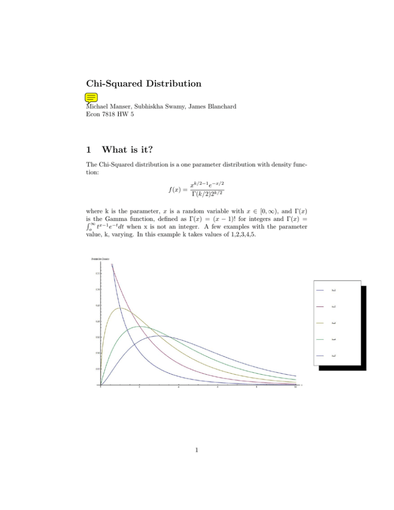
Chi-Squared Distribution
Michael Manser, Subhiskha Swamy, James Blanchard
Econ 7818 HW 5
1
What is it?
The Chi-Squared distribution is a one parameter distribution with density function:
f (x) =
xk/2−1 e−x/2
Γ(k/2)2k/2
where k is the parameter, x is a random variable with x ∈ [0, ∞), and Γ(x)
is
Gamma function, defined as Γ(x) = (x − 1)! for integers and Γ(x) =
R ∞thex−1
t
e−t dt when x is not an integer. A few examples with the parameter
o
value, k, varying. In this example k takes values of 1,2,3,4,5.
1
In the next example k = 10,15,20.
The cumulative distribution function for the Chi-Squared distribution is
given by:
F (x; k) =
γ(k/2, x/2)
= P (k/2, x/2)
Γ(k/2)
Where
x) is the lower incomplete gamma function defined by γ(a, x) =
R x a−1 γ(a,
−t
t
e
dt.
0
2
Again, a few examples of the Chi-Squared CDF at k = 1,2,3,4,5.
3
2
Where does it come from and why is it useful?
This is Karl Pearson (1857-1936), the father of modern statistics (establishing the first statistics department in the world at University College London)
and the man who came up with the Chi-Squared distribution. Pearson’s work
in statistics began with developing mathematical methods for studying the processes of heredity and evolution (leading to his aggressive advocacy of eugenics).
The Chi-Squared distribution came about as Pearson was attempting to find a
measure of the goodness of fit of other distributions to random variables in
his heredity and evolutionary modelling. Also note that Ernst Abbe wrote his
dissertation in 1863 deriving the Chi-Square distribution, although he switched
fields soon after the publication of the paper to optics and astronomy.
It turns out that the Chi-Square is one of the most widely used distributions in
inferential statistics. So understanding the Chi-Square distribution is important
for hypothesis testing, constructing confidence intervals, goodness of fit, Friedman’s analysis of variance by ranks, etc. The distribution is also important in
discrete hedging of options in finance, as well as option pricing.
4
2.1
Measures of Central Tendency
The mean, median, mode and variance for the Chi-Squared distribution are:
M ean = k
2 2
)
9k
M ode = max(k − 2, 0)
M edian = k(1 −
2.2
Moment Generating Function
We know that for a continuous distribution the moment generating function
takes the general form:
Z ∞
M (t) =
ext f (x)dx
−∞
Thus plugging in the Chi-Squared density function and integrating yields
the moment generating function for the Chi-Squared distribution:
M (t) = (1 − 2t)−k/2
From the moment generating function we can find out lots of information
about the Chi-Squared distribution:
M 0 (t) = (k)(1 − 2t)−k/2−1 ⇒ M 0 (0) = k
which is the mean. Using the same procedure1 one can find the variance, skewness, kurtosis, etc.
V ariance = 2k
p
Skewness = 8/k
Kurtosis = 3 + 12/k
The graph below provides an illustration of the skewness and kurtosis of the ChiSquared distribution as the parameter, k, changes. The blue graph represents
k = 3, and the red graph represents k = 10.
1 Note that the first four moments (and perhaps more) can be found using
Mathematica.
The function for Mathematica are Mean[ChiSquareDistribution[k]],
Variance[ChiSquareDistribution[k]],
Skewness[ChiSquareDistribution[k]],
and Kurtosis[ChiSquareDistribution[k]]
5
The mean and variance are positively related to k, so the red graph has a higher
mean and variance than the blue graph. Skewness and kurtosis, on the other
hand, are inversely related to k, so the red graph has a lower skewness and
kurtosis than the blue graph2 .
If we think of skewness as how symmetric the distribution is around the mode,
with perfect symmetry as skewness approaches zero, clearly the red PDF is much
more symmetric than the blue PDF. Notice how the skewness of the density
function changes with values of k, but the curve remains positively skewed. We
can think of kurtosis as the ”flatness” of the curve around the mode, so the
high kurtosis means that the curve will be very steep around the mode. Again,
the red and blue graphs illustrate this concept, with the red graph being much
flatter than the blue graph around the mode. Another way to think of kurtosis
is that the ”tails are fatter” when the kurtosis is low.
2 We
can even calculate these to prove it. skewnessblue = 1.633 and skewnessred = 0.894,
kurtosisblue = 7 and kurtosisred = 4.2
6
In the next example k = 50 and k = 100. Notice that as k increases, the
PDF tends to flatten out.
As k approaches ∞ the PDF tends to resemble the normal distribution, which
is a result of the Central Limit Theorem3 .
3 We shall show by the Central Limit Theorem that the Chi-Squared distribution resembles
Pn
the Normal distribution as k approaches ∞. So let Yi ∼ χ21 , thus
Y ∼ χ2n . Therefore,
i=1 i
Pn
i=1
by the Central Limit Theorem,
Thus
χ2
n
√
n 2
−
1
√
2
→ N (0, 1) so
Yi −nE(Yi )
σ
χ2n
→
N (n, 2n2 )
7
→ N (0, 1) which becomes
χ2 −n
√n √
2n n
→ N (0, 1).
3
Examples
Example 1
Suppose we are trying to asses the property damage that results from the flooding of a river. It is reasonable to suppose that the damage will be worse closer
to the river. In this case it is reasonable to expect that if damage is a function of
distance from the river, it may be Chi-Squared distributed with the parameter
k=1. The following graph illustrates how property damage may be distributed
according to distance. Other scenarios possibly represented by this distribution
include the value of a Boulder home as a function of distance to official ”open
space”.
8
Example 2
Now suppose that we are trying to find a distribution that represents the age
that an individual contracts HIV from sexual activity. We go out and ask every person with HIV at what age they contracted the virus. With our data
we then randomly draw samples from the uniform distribution. After enough
draws we should see the mean tending to 30 years. Thus our distribution may
be Chi-Squared distributed with k = 30. This seems reasonable since it is very
unlikely that many children will have gotten HIV through sexual activity, and
presumably the older someone gets the less promiscuous they are. Thus the risk
of contracting HIV declines as an individual ages.
Example 3
Say we were interested in modelling the amount of alcohol (measured in litres)
that the average American who does, in fact, drink consumes per year. Since we
are excluding all Americans who do not drink (children, certain religious groups,
etc.) it is reasonable to assume that the probability of one of these individuals
consuming no alcohol per year is zero, or else they would be excluded from our
population. We also know that as the litres consumed increases to infinity, the
probability decreases, since alcohol in vast quantities has some peculiar side effects, most importantly, death. Perhaps we would want to use the Chi-Square
distribution for this model. As long as k is not one or two, the probability at
zero is zero, and the probability tends to zero as x approaches infinity. Since
the average annual consumption of alcohol per capita is around 6 litres, but this
population includes non-drinkers, so perhaps we decide to increase the number
of litres by 1. So we believe that the mean of our population is 7 litres per
9
year, per person who drinks. The data generating process for this distribution
is similar to the HIV data generating process. We simply draw individuals who
drink from a uniform distribution and record the amount of alcohol they consume per year. After enough draws the distribution should tend towards the
Chi-Squared. Since the mean of the Chi-Squared is equal to k, we know our
parameter value. Plotting the PDF for k = 6 yields:
A few more examples
The PDF for one and three dimensional fields in a mode-stirred chamber is ChiSquared distributed. ”Statistical methods for a mode-stirred chamber”, Kostas
and Boverie, IEEE Transactions on Electromagnetic Compatibility, 2002.
In detecting a deterministic signal in white Gaussian noise by means of an
energy measuring device, the decision statistic is chi-squared distributed when
the signal is absent, and noncentral Chi-Squared distributed when the signal
is present. ”Energy detection of unknown deterministic signals”, Urkowitz,
Proceedings of the IEEE, 2005.
The constant elasticity of variance options pricing formula can be represented
by the noncentral Chi-Squared distribution. ”Computing the constant elasticity
of variance options pricing formula”, Schroeder, Journal of Finance, 1989.
The conditional distribution of the short rate in the Cox-Ingersoll-Ross process can be represented by the noncentral Chi-Squared distribution. ”Evaluating the noncentral Chi-Squared distribution for the Cox-Ingersoll-Ross process”,
10
Dyrting, Computational Economics, 2004.
11
4
Other Distributions?
There are many distributions that are similar to the Chi-Squared. The Poisson
distribution resembles a discrete version of the Chi-Squared. Like the ChiSquared, the Poisson is a one parameter distribution and has the same shape as
the Chi-Squared. The following example is a Poisson distribution with k = 3.
12
Another example where k = 5. Notice how the distribution takes the same
shape as the Chi-Squared.
13
Another distribution that is similar to the Chi-Squared is the Weibull distribution, which is a two parameter continuous distribution. In the following
example λ = 2 and n = 2.
5
Proof That Square of Normal is Chi-Squared
The following proof is of interest since it shows the direct relationship between
the Normal distribution and the Chi-Squared distribution. If X ∼ N (0, 1), we
will show that X 2 ∼ Chi-Squared distribution with k = 1.
To find the distribution of X 2 , we write the CDF of X 2 as:
FX 2 (a) = P (x2 ≤ a)
√
√
P (− a ≤ x ≤ a if a > 0;
=
0
if a ≤ 0.
for all a ≥ 0,
√
√
FX 2 (a) = FX ( a) − FX (− a)
This result is derived in the sampling distribution notes. Differentiation with
respect to a, we get the density function:
√ a−1/2
√ −a−1/2
− fX (− a)
fX 2 (a) = fX ( a)
2
2
=
√
√
a−1/2
(fX ( a) + fX (− a))
2
14
6
=
1
a−1/2
2 √ e−a/2
2
2π
=
( 21 )1/2 a−1/2 e−a/2
p
1/2
Chi-Squared Tests
A Chi-Squared test is any hypothesis test where the sampling distribution of
the test statistic is Chi-Squared distributed when the null hypothesis is true.
Perhaps the most well known example of a Chi-Squared test is Pearson’s ChiSquared test, which tests the null that the distribution of the sample is consistent
with a specific theoretical distribution. Other examples of Chi-Squared tests
include Ljung-Box, Box-Pierce, and other portmanteau tests which test the
stationarity of time-series data.
References
[1] Introduction to the Theory of Statistics - Mood, Graybill, Boes
[2] Alcohol Consumption - http://www.greenfacts.org/en/alcohol/figtableboxes/figure3.htm
[3] Chi-Squared, WolframMathworld - http://mathworld.wolfram.com/ChiSquaredDistribution.html
[4] Wikipedia - Chi-Squared Distribution, Chi-Squared Tests, Gamma Function, Karl Pearson, Ernst Abbe
[5] The Chi-Squared Distribution, Harpreet Bedi, Chad Garnett, Wooyoung
Park
[6] A bit on sampling distributions, Edward Morey
15