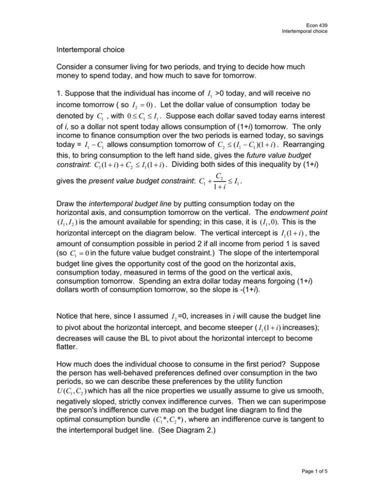
Econ 439
Intertemporal choice
Intertemporal choice
Consider a consumer living for two periods, and trying to decide how much
money to spend today, and how much to save for tomorrow.
1. Suppose that the individual has income of I1 >0 today, and will receive no
income tomorrow ( so I 2 = 0) . Let the dollar value of consumption today be
denoted by C1 , with 0 ≤ C1 ≤ I1 . Suppose each dollar saved today earns interest
of i, so a dollar not spent today allows consumption of (1+i) tomorrow. The only
income to finance consumption over the two periods is earned today, so savings
today = I1 − C1 allows consumption tomorrow of C2 ≤ ( I1 − C1 )(1 + i ) . Rearranging
this, to bring consumption to the left hand side, gives the future value budget
constraint: C1 (1 + i ) + C2 ≤ I1 (1 + i ) . Dividing both sides of this inequality by (1+i)
gives the present value budget constraint: C1 +
C2
≤ I1 .
1+ i
Draw the intertemporal budget line by putting consumption today on the
horizontal axis, and consumption tomorrow on the vertical. The endowment point
( I1 , I 2 ) is the amount available for spending; in this case, it is ( I1 , 0). This is the
horizontal intercept on the diagram below. The vertical intercept is I1 (1 + i ) , the
amount of consumption possible in period 2 if all income from period 1 is saved
(so C1 = 0 in the future value budget constraint.) The slope of the intertemporal
budget line gives the opportunity cost of the good on the horizontal axis,
consumption today, measured in terms of the good on the vertical axis,
consumption tomorrow. Spending an extra dollar today means forgoing (1+i)
dollars worth of consumption tomorrow, so the slope is -(1+i).
Notice that here, since I assumed I 2 =0, increases in i will cause the budget line
to pivot about the horizontal intercept, and become steeper ( I1 (1 + i ) increases);
decreases will cause the BL to pivot about the horizontal intercept to become
flatter.
How much does the individual choose to consume in the first period? Suppose
the person has well-behaved preferences defined over consumption in the two
periods, so we can describe these preferences by the utility function
U (C1 , C2 ) which has all the nice properties we usually assume to give us smooth,
negatively sloped, strictly convex indifference curves. Then we can superimpose
the person's indifference curve map on the budget line diagram to find the
optimal consumption bundle (C1 *, C2 *) , where an indifference curve is tangent to
the intertemporal budget line. (See Diagram 2.)
Page 1 of 5
Econ 439
Intertemporal choice
At the optimal consumption bundle, the slope of an indifference curve is just
equal to the slope of the budget line. In this particular context, this means that at
the optimal consumption bundle, an individual's psychic rate of trade-off between
consumption today and consumption tomorrow, given by their rate of time
preference, is equated to the market rate of tradeoff, given by the interest rate.
What happens to the optimal consumption bundle if i increases? Then
consumption today becomes more expensive relative to consumption tomorrow,
and the substitution effect says that consumption tomorrow should go up. On the
other hand, a given amount of savings today will finance more consumption
tomorrow, so an increase in the interest rate makes a person wealthier - the
income effect also says consumption tomorrow should go up. What about
consumption today? Income and substitution effects work in opposite directions,
so the effect is ambiguous.
2. Now suppose that the individual has strictly positive income in both periods.
The only change to the analysis above is that the endowment point,
E= ( I1 , I 2 ) , is now a point in the positive quadrant rather than on the horizontal
axis. Changes in the interest rate will, as before, pivot the intertemporal
budget line about the endowment point, but the analysis is slightly more
complicated now. The intertemporal budget constraint now includes
consideration of the second period positive income. The future value budget
constraint is C1 (1 + i ) + C2 ≤ I1 (1 + i ) + I 2 , while the present value version is
C1 +
C2
I
≤ I1 + 2 .
1+ i
1+ i
Consider Diagram 3 below. Here I have assumed positive income in both
periods, and allowed for borrowing as well as lending at the common interest rate
i.
Now the person can be a borrower ( C1 > I1 , C2 < I 2 ) ) or a lender
( C1 < I , C2 > I 2 ) depending on preferences. Consider the indifference curve
through the endowment point - this represents the utility the individual would
have if they consumed their income in each period, neither borrowing nor
lending. If this indifference curve through E is steeper than the budget line, then
the individual would be better off borrowing against period 2 income to increase
consumption in period 1 - because they have a high rate of time preference (or,
some say, are impatient). For this person, the tangency of the budget line and
an indifference curve occurs on the budget line below E.
Conversely, a person will be a lender if their indifference curve through E is flatter
than the intertemporal budget line at point E.
Page 2 of 5
Econ 439
Intertemporal choice
Now: comparative statics: what can we say about the effects of a change in the
interest rate on the amount a person borrows or lends? As in the first case I
described, some predictions are ambiguous and some are unambiguous.
Suppose at the initial income stream ( I1 , I 2 ) and interest rate i, Rae is a
borrower, as in the diagram below, initially consuming at point A= (C1 A , C2 A ) below
E on the intertemporal budget line. An increase in the interest rate to i ' > i pivots
the budget line through E, making it steeper, with a higher vertical intercept
I
I
( I1 (1 + i ) + I 2 < I1 (1 + i ') + I 2 ) and a lower horizontal intercept ( I1 + 2 < I1 + 2 )
1+ i
1+ i'
than with the initial interest rate. Notice that bundle A is no longer attainable,
since it is outside the new budget set. An increase in the interest rate will induce
a borrower to borrow less, and may even turn a borrower into a lender.
How does Rae's optimal bundle change when the interest rate decreases?
Bundle A is still attainable, but no longer optimal, since it is now inside the budget
set. The new optimal bundle will be on the new budget line, and may have
increased consumption in both periods.
Page 3 of 5
Econ 439
Intertemporal choice
Diagram 1
Consumption
in pd 2
I1 (1 + i )
(0,0)
I1
Consumption in pd 1
Diagram 2
Consumption
in pd 2
I1 (1 + i )
(C1 *, C2 *)
(0,0)
I1
Consumption in pd 1
Page 4 of 5
Econ 439
Intertemporal choice
Diagram 3
Consumption in pd 2
I 2 + I1 (1 + i )
E
I2
A
0,0
I1
I
I
1 +
2
1+ i'
I
I
1 +
2
1+ i
Consumption in pd 1
Page 5 of 5