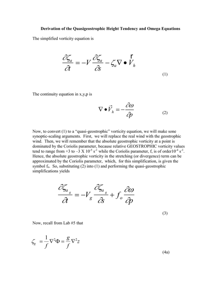
Derivation of the Quasigeostrophic Height Tendency and Omega Equations
The simplified vorticity equation is
r
a
a
 V
 a   Vh
t
s
(1)
The continuity equation in x,y,p is

 Vh  

p
(2)
Now, to convert (1) to a “quasi-geostrophic” vorticity equation, we will make sone
synoptic-scaling arguments. First, we will replace the real wind with the geostrophic
wind. Then, we will remember that the absolute geostrophic vorticity at a point is

dominated by the Coriolis parameter, because relative GEOSTROPHIC vorticity values
tend to range from +3 to –3 X 10-5 s-1 while the Coriolis parameter, f, is of order10-4 s-1.
Hence, the absolute geostrophic vorticity in the stretching (or divergence) term can be
approximated by the Coriolis parameter, which, for this simplification, is given the
symbol fo. So, substituting (2) into (1) and performing the quasi-geostrophic
simplifications yields
a
a

 Vg
 fo
t
s
p
g
g
(3)
Now, recall from Lab #5 that

g 
1 2
g
   2z
f
f
(4a)

a g 
1 2
g
   f  2z  f
f
f
(4b)
where ø =-gz.

Substituting (4) into the left side of (3), remembering that the local tendency of f = 0 and
expanding the absolute vorticity in the advection term, yields
 2
2 
 V g  ( g  f )  f o
t
p
(5)
Quasigeostrophic Vorticity Equation
 where the vector notation is used for the horizontal advection term.
This is the
quasigeostrophic vorticity equation. It is valid to the extent that the wind is geostrophic
and that the simplifications made to the vorticity equation based upon synoptic scaling
apply.
The thermodynamic energy equation is
T
T
dQ
T  v T  
 
 

u
t
x
y
c pT
dt
 p
t
 u T
x
 v T

p 
 1 dQ


y
cp
dt
 R
(6a,b)
We can substitute the equation of state into the hydrostatic law




T  p R   p


(7)
and place (7) into (6). Equation (7) states that the temperature is proportional to the
mean thickness of the layer centering on the level in quesiton. We can also assume that
diabatic effects are small, substitute in the definition of the static stability parameter, and
assume that hat the wind is geostrophic to obtain the quasigeostrophic thermodynamic
energy equation,.

 p  

 V g  T   p

R
t  R  p
2

(8)
Quasigeostrophic thermodynamic energy equation
We can simplify the left hand side of (8) by remembering that

 





t



 

t  p
p

 
 
 t 
(9a,b)
where X is the geopotential height tendency (X<0 = height falls etc.). Equations (9a,b)
can be substituted into equations (5) and (8) to obtain the final form of the quasigeostrophic vorticity and thermodynamic energy equations. (Equations 5.6.5 and 5.6.6 on
page 328 of Bluestein).

 2    f o V g  (g  f )  f o 2

p
(10)



 p R  p  Vg  T   p R
(11)
Multiply (11) by -(fo2) R/p and differentiate with respect to pressure,

f o2  2

f o2 
2 
Vg  T  f o
2 
p
 p
p


(12)
Now add (12) to (10) and rearrange terms to obtain the quasigeostrophic height
tendency equation.

3
 2 f 2 2 
f o 2  R

o 
V

T
 
2    f o V g  ( g  f o ) 
g
 p
(12)

 p 
 p 



Quasigeostrophic Height Tendency Equation

Please note that in many derivations, equation (7) is substituted into the temperature
advection term. In that case, the temperature advection is appxoximated by the thickness
advection by the geosgrophic wind.
Multiply Equation (11) by (R/p) and then take the Laplacian of the result. Multiply
Equation (10) by by -(fo) and differentiate the result with respect to pressure (∂/∂p).
Subtracting (10) from (11) and collecting terms yields the quasigeostrophic omega
equation.
 2 f 2 2 
f o2 
o 
V g  ( g  f )  R p  2 V g  T
 
2   
 p 
 p




 (13)
Quasigeostrophic Omega Equation

Equations (12) and (13) can be rederived neglecting the assumption that diabatic effects
are minimal. As Bluestein points out on pp. 328-330 this assumption is a bad one near
the surface where diurnal sensible heating/cooling effects can be large, at cloud top level
when radiational effects might be large, and, when latent heat releases associated with
cloud development.
2
 2 f 2 2 
f o 2  R
 f o  R  1 dQ 
o 

 
2    f o V g  ( g  f ) 

 p Vg  T 
  p 
dt 

 p 
 p 
 p  c p



(14) Quasigeostrophic Height Tendency Equation With Diabatic Term

 2 f 2 2 


f o2 
o 





V g  ( g  f )  R p  2 Vg  T  R p  2 1c dQ dt 

2 
 p

 p 
 p





(15) Quasigeostrophic Omega Equation With Diabatic Term

4
Interpretation of the Quasigeostrophic Equations
The left hand side of the two equations contains a term that has the appearance of a threedimensional Laplacian. The term can be estimated analytically, for example, when the
user of the equation is attempting to evaluate the equations, say, for a 500 mb pattern
with troughs and ridges. The pattern of omega is also sinusoidal. The exact evaluation
will be left to Metr 520 (Dymamic Meteorology II), and reduces to a constant
 2 f 2 2
  2 2 1  f  2 
o 
o
 
   C
2  k  l 

p


 p  

 



where k and l are constants dependent upon wavelength and amplitude of the disturbance
at a given pressure level p. Applying (15) to the left hand sides of equations (13) and
(14) allows one to make the assumption that
   f o V g  ( g  f ) 
|

(16)
2
f o 2  R
 f o  R  1 dQ 
V

T



 p g
  p 
dt 


 p 
 p  c p


“Dynamic Effects”
“Thermal Effects”
|
(17) Simplified Quasigeostrophic Height Tendency Equation With Diabatic Term
and


f o2 
  
V g  ( g  f )  R  2 Vg  T  R  2  1 dQ 
p
p  c p dt 
 p

|



“Dynamic Effects”
“Thermal Effects”
|

(18) Simplified Quasigeostrophic Omega Equation With Diabatic Term
The tendency equation (prognostic) states that height falls at a given location on a
pressure surface (say, 500 mb) when, at that location, positive (or cyclonic) vorticity
advection occurs, and/or cold advection decreasing with height (known as differential
temperature advection), and/or sensible chilling decreasing with height (differential
diabatic temperature change).
5
The omega equation (diagnostic) states that upward motion at a given location on a
pressure surface (say, 500 mb) is associated with vorticity advection becoming more
cyclonic with height (known as differential vorticity advection), and/or a warm advection
maximum is located at that point, and/or a sensible heating maximum is located at that
point.
6