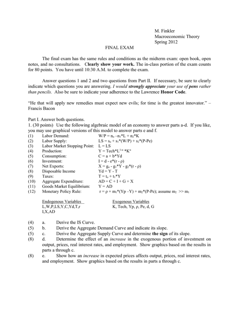
M. Finkler
Macroeconomic Theory
Spring 2012
FINAL EXAM
The final exam has the same rules and conditions as the midterm exam: open book, open
notes, and no consultations. Clearly show your work. The in-class portion of the exam counts
for 80 points. You have until 10:30 A.M. to complete the exam.
Answer questions 1 and 2 and two questions from Part II. If necessary, be sure to clearly
indicate which questions you are answering. I would strongly appreciate your use of pens rather
than pencils. Also be sure to indicate your adherence to the Lawrence Honor Code.
“He that will apply new remedies must expect new evils; for time is the greatest innovator.” –
Francis Bacon
Part I. Answer both questions.
1. (30 points) Use the following algebraic model of an economy to answer parts a-d. If you like,
you may use graphical versions of this model to answer parts e and f.
(1)
(2)
(3)
(4)
(5)
(6)
(7)
(8)
(9)
(10)
(11)
(12)
Labor Demand:
Labor Supply:
Labor Market Stopping Point:
Production:
Consumption:
Investment:
Net Exports:
Disposable Income
Taxes:
Aggregate Expenditure:
Goods Market Equilibrium:
Monetary Policy Rule:
Endogenous Variables
L,W,P,LS,Y,C,Yd,T,r
I,X,AD
(4)
(5)
(5)
(8)
(8)
W/P = no –n1*L + n2*K
LS = so + s1*(W/P) + s2*(P-Pe)
L = LS
Y = Tech*L1-α *Kα
C = a + b*Yd
I = d - e*(r - ρ)
X = go - g1*Y - g2*(r - ρ)
Yd = Y - T
T = to + t1*Y
AD = C + I + G + X
Y = AD
r = ρ + m1*(Yp –Y) + m2*(P-Pe); assume m2 >> m1
Exogenous Variables
K, Tech, Yp, ρ, Pe, d, G
a.
Derive the IS Curve.
b.
Derive the Aggregate Demand Curve and indicate its slope.
c.
Derive the Aggregate Supply Curve and determine the sign of its slope.
d.
Determine the effect of an increase in the exogenous portion of investment on
output, prices, real interest rates, and employment. Show graphics based on the results in
parts a through c.
e.
Show how an increase in expected prices affects output, prices, real interest rates,
and employment. Show graphics based on the results in parts a through c.
2. (20 points) Consider the following version of model 5. All variables with the exception of the
inflation-related variables are expressed in current year terms; so the “t” subscript has been
suppressed except for those variables.
.
IS Curve: Y = Yp – α*r + G + є with є a random shock variable
Fisher Equation: r = i - πet+1
Phillips Curve: πt = πet + φ(Y – Yp) + v
with v a random shock variable
Inflation Expectations: πet = πt-1
Monetary Policy: i = π + ρ + θ*(π – π*) + (1- θ)*(Y-Yp)
Endogenous variables: Y, r, π, πe, i
Exogenous variables: Yp, ρ, G, v, є, π*
(6) a.
Derive the dynamic aggregate demand curve. Indicate its slope.
(2) b.
Determine the dynamic aggregate supply curve and indicate its slope.
(6) c.
Show (graphically) the effects of a temporary increase in the natural rate of
interest on the paths of output and inflation.
(6) d.
Show (graphically) the effects of a permanent decrease in governmental
purchases on the paths of output and inflation.
Part II (15 points each) Answer two of the following questions.
1. Use Model 4 or Model 5 to illustrate and explain why activist monetary policy can clearly
improve economic performance if there is a demand shock but requires a tradeoff of
policy objectives if there is a supply shock.
2. Use Model 4 to illustrate and explain the effects of an exogenous decline in raw material
prices on GDP, employment, prices, real wages, and interest rates. (Assume that the
decline in raw materials prices leads to increased purchases of raw materials.)
3. Given the current state of the Eurozone economy, assume that there is increased
uncertainty with regard to the value of the debt instruments issued by many Eurozone
countries and, thus, on the Eurozone as a whole. Use the Mundell-Fleming Model to
illustrate and explain the effects of such increased uncertainty on Eurozone GDP, interest
rates, trade balances, and exchange rates. Assume that Euro floats against other
currencies and that the Eurozone follows large country assumptions. What might cause
these results not to take place?
4. Use the standard Solow growth model (1g) with exogenous technical change that grows
at g% per year. How would a fall in the savings rate affect steady state income per capita
and the capital/labor ratio? Support your answer either algebraically or graphically.