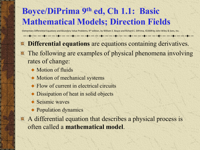
Boyce/DiPrima 9th ed, Ch 1.1: Basic
Mathematical Models; Direction Fields
Elementary Differential Equations and Boundary Value Problems, 9th edition, by William E. Boyce and Richard C. DiPrima, ©2009 by John Wiley & Sons, Inc.
Differential equations are equations containing derivatives.
The following are examples of physical phenomena involving
rates of change:
Motion of fluids
Motion of mechanical systems
Flow of current in electrical circuits
Dissipation of heat in solid objects
Seismic waves
Population dynamics
A differential equation that describes a physical process is
often called a mathematical model.
Example 1: Free Fall
Formulate a differential equation describing motion of an
object falling in the atmosphere near sea level.
Variables: time t, velocity v
Newton’s 2nd Law: F = ma = m(dv/dt) net force
Force of gravity: F = mg
downward force
Force of air resistance: F =  v
upward force
Then
dv
m  mg   v
dt
Taking g = 9.8 m/sec2, m = 10 kg,  = 2 kg/sec,
we obtain dv
dt
 9.8  0.2v
v  9.8  0.2v
Example 2: Sketching Direction Field (1 of 3)
Using differential equation and table, plot slopes (estimates)
on axes below. The resulting graph is called a direction
field. (Note that values of v do not depend on t.)
v
0
5
10
15
20
25
30
35
40
45
50
55
60
v'
9.8
8.8
7.8
6.8
5.8
4.8
3.8
2.8
1.8
0.8
-0.2
-1.2
-2.2
Example 2:
Direction Field Using Maple (2 of 3)
v  9.8  0.2v
Sample Maple commands for graphing a direction field:
with(DEtools):
DEplot(diff(v(t),t)=9.8-v(t)/5,v(t),
t=0..10,v=0..80,stepsize=.1,color=blue);
When graphing direction fields, be sure to use an
appropriate window, in order to display all equilibrium
solutions and relevant solution behavior.
v  9.8  0.2v
Example 2:
Direction Field & Equilibrium Solution (3 of 3)
Arrows give tangent lines to solution curves, and indicate
where soln is increasing & decreasing (and by how much).
Horizontal solution curves are called equilibrium solutions.
Use the graph below to solve for equilibrium solution, and
then determine analytically by setting v' = 0.
Set v  0 :
 9.8  0.2v  0
9.8
v
0.2
 v  49
Equilibrium Solutions
In general, for a differential equation of the form
y  ay  b,
find equilibrium solutions by setting y' = 0 and solving for y :
y (t ) 
b
a
Example: Find the equilibrium solutions of the following.
y  2  y
y  5 y  3
y  y ( y  2)
Example 3: Mice and Owls (1 of 2)
Consider a mouse population that reproduces at a rate
proportional to the current population, with a rate constant
equal to 0.5 mice/month (assuming no owls present).
When owls are present, they eat the mice. Suppose that
the owls eat 15 per day (average). Write a differential
equation describing mouse population in the presence of
owls. (Assume that there are 30 days in a month.)
Solution:
dp
 0.5 p  450
dt
Example 5: Direction Field (2 of 2)
Discuss solution curve behavior, and find equilibrium soln.
p  0.5 p  450
Steps in Constructing Mathematical Models
Using Differential Equations
Identify independent and dependent variables and assign
letters to represent them.
Choose the units of measure for each variable.
Articulate the basic principle that underlies or governs the
problem you are investigating. This requires your being
familiar with the field in which the problem originates.
Express the principle or law in the previous step in terms of
the variables identified at the start. This may involve the use
of intermediate variables related to the primary variables.
Make sure each term of your equation has the same physical
units.
The result may involve one or more differential equations.