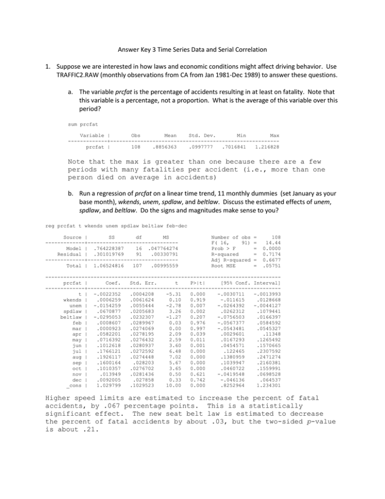
Answer Key 3 Time Series Data and Serial Correlation
1. Suppose we are interested in how laws and economic conditions might affect driving behavior. Use
TRAFFIC2.RAW (monthly observations from CA from Jan 1981-Dec 1989) to answer these questions.
a. The variable prcfat is the percentage of accidents resulting in at least on fatality. Note that
this variable is a percentage, not a proportion. What is the average of this variable over this
period?
sum prcfat
Variable |
Obs
Mean
Std. Dev.
Min
Max
-------------+-------------------------------------------------------prcfat |
108
.8856363
.0997777
.7016841
1.216828
Note that the max is greater than one because there are a few
periods with many fatalities per accident (i.e., more than one
person died on average in accidents)
b. Run a regression of prcfat on a linear time trend, 11 monthly dummies (set January as your
base month), wkends, unem, spdlaw, and beltlaw. Discuss the estimated effects of unem,
spdlaw, and beltlaw. Do the signs and magnitudes make sense to you?
reg prcfat t wkends unem spdlaw beltlaw feb-dec
Source |
SS
df
MS
-------------+-----------------------------Model | .764228387
16 .047764274
Residual | .301019769
91
.00330791
-------------+-----------------------------Total | 1.06524816
107
.00995559
Number of obs
F( 16,
91)
Prob > F
R-squared
Adj R-squared
Root MSE
=
=
=
=
=
=
108
14.44
0.0000
0.7174
0.6677
.05751
-----------------------------------------------------------------------------prcfat |
Coef.
Std. Err.
t
P>|t|
[95% Conf. Interval]
-------------+---------------------------------------------------------------t | -.0022352
.0004208
-5.31
0.000
-.0030711
-.0013993
wkends |
.0006259
.0061624
0.10
0.919
-.011615
.0128668
unem | -.0154259
.0055444
-2.78
0.007
-.0264392
-.0044127
spdlaw |
.0670877
.0205683
3.26
0.002
.0262312
.1079441
beltlaw | -.0295053
.0232307
-1.27
0.207
-.0756503
.0166397
feb |
.0008607
.0289967
0.03
0.976
-.0567377
.0584592
mar |
.0000923
.0274069
0.00
0.997
-.0543481
.0545327
apr |
.0582201
.0278195
2.09
0.039
.0029601
.11348
may |
.0716392
.0276432
2.59
0.011
.0167293
.1265492
jun |
.1012618
.0280937
3.60
0.001
.0454571
.1570665
jul |
.1766121
.0272592
6.48
0.000
.122465
.2307592
aug |
.1926117
.0274448
7.02
0.000
.1380959
.2471274
sep |
.1600164
.028203
5.67
0.000
.1039947
.2160381
oct |
.1010357
.0276702
3.65
0.000
.0460722
.1559991
nov |
.013949
.0281436
0.50
0.621
-.0419548
.0698528
dec |
.0092005
.027858
0.33
0.742
-.046136
.064537
_cons |
1.029799
.1029523
10.00
0.000
.8252964
1.234301
Higher speed limits are estimated to increase the percent of fatal
accidents, by .067 percentage points. This is a statistically
significant effect. The new seat belt law is estimated to decrease
the percent of fatal accidents by about .03, but the two-sided p-value
is about .21.
Interestingly, increased economic activity also increases the percent
of fatal accidents. This may be because more commercial trucks are on
the roads, and these probably increase the chance that an accident
results in a fatality.
c. Test the errors for AR(1) serial correlation.
Here is how you could conduct the test using the Breusch-Godfrey
method: After getting the OLS residuals, uˆt , run the regression
uˆt on uˆt 1 , t  2,...,108.
(Included an intercept, but that is unimportant.)
tsset t
predict error, resid
reg error l.error
Source |
SS
df
MS
-------------+-----------------------------Model | .023534599
1 .023534599
Residual | .277302016
105 .002640972
-------------+-----------------------------Total | .300836614
106 .002838081
Number of obs
F( 1,
105)
Prob > F
R-squared
Adj R-squared
Root MSE
=
=
=
=
=
=
107
8.91
0.0035
0.0782
0.0695
.05139
-----------------------------------------------------------------------------error |
Coef.
Std. Err.
t
P>|t|
[95% Conf. Interval]
-------------+---------------------------------------------------------------error |
L1. |
.2816415
.0943463
2.99
0.004
.0945701
.4687129
_cons |
.0002981
.0049684
0.06
0.952
-.0095533
.0101496
The coefficient on uˆt 1 is ̂  .281 (se = .094).
Thus, there is
evidence of some positive serial correlation in the errors (t  2.99).
Note that this test is only valid if there are no concerns about the
endogeneity of the regressors. A strong case can be made that all
explanatory variables are strictly exogenous. Certainly there is no
concern about the time trend, the seasonal dummy variables, or wkends,
as these are determined by the calendar. It is seems safe to assume
that unexplained changes in prcfat today do not cause future changes
in the state-wide unemployment rate. Also, over this period, the
policy changes were permanent once they occurred, so strict exogeneity
seems reasonable for spdlaw and beltlaw. (Given legislative lags, it
seems unlikely that the dates the policies went into effect had
anything to do with recent, unexplained changes in prcfat.
d. Re-estimate the model accounting to serial correlation.
Couple of options:
. arima prcfat t wkends unem spdlaw beltlaw feb-dec, ar(1)
(setting optimization to BHHH)
Iteration 0:
log likelihood =
Iteration 1:
log likelihood =
Iteration 2:
log likelihood =
168.775
168.81849
168.85351
Iteration 3:
log likelihood =
Iteration 4:
log likelihood =
(switching optimization to BFGS)
Iteration 5:
log likelihood =
Iteration 6:
log likelihood =
Iteration 7:
log likelihood =
Iteration 8:
log likelihood =
Iteration 9:
log likelihood =
Iteration 10: log likelihood =
Iteration 11: log likelihood =
168.8576
168.85947
168.86032
168.8641
168.86419
168.86439
168.8644
168.8644
168.8644
ARIMA regression
Sample:
1 - 108
Log likelihood =
168.8644
Number of obs
Wald chi2(17)
Prob > chi2
=
=
=
108
191.09
0.0000
-----------------------------------------------------------------------------|
OPG
prcfat |
Coef.
Std. Err.
z
P>|z|
[95% Conf. Interval]
-------------+---------------------------------------------------------------prcfat
|
t | -.0021501
.0005349
-4.02
0.000
-.0031986
-.0011017
wkends |
.0006179
.0054809
0.11
0.910
-.0101244
.0113602
unem | -.0132124
.0068961
-1.92
0.055
-.0267285
.0003037
spdlaw |
.0641854
.0298944
2.15
0.032
.0055935
.1227773
beltlaw | -.0248763
.0338792
-0.73
0.463
-.0912783
.0415257
feb | -.0008934
.0361499
-0.02
0.980
-.071746
.0699591
mar | -.0011545
.0306679
-0.04
0.970
-.0612625
.0589534
apr |
.0575487
.0315385
1.82
0.068
-.0042656
.1193629
may |
.0718131
.0263242
2.73
0.006
.0202186
.1234076
jun |
.1007231
.0252368
3.99
0.000
.0512599
.1501863
jul |
.174789
.0225581
7.75
0.000
.1305759
.2190022
aug |
.1919537
.0308971
6.21
0.000
.1313964
.252511
sep |
.159901
.0287129
5.57
0.000
.1036247
.2161772
oct |
.1007692
.0243195
4.14
0.000
.0531039
.1484345
nov |
.0133081
.0275731
0.48
0.629
-.0407342
.0673504
dec |
.0085411
.0281464
0.30
0.762
-.0466249
.0637071
_cons |
1.009016
.1103693
9.14
0.000
.7926966
1.225336
-------------+---------------------------------------------------------------ARMA
|
ar |
L1. |
.2859698
.1117903
2.56
0.011
.0668649
.5050747
-------------+---------------------------------------------------------------/sigma |
.0506463
.0041883
12.09
0.000
.0424375
.0588551
Or this one:
. prais prcfat t wkends unem spdlaw beltlaw feb-dec
Iteration
Iteration
Iteration
Iteration
Iteration
Iteration
0:
1:
2:
3:
4:
5:
rho
rho
rho
rho
rho
rho
=
=
=
=
=
=
0.0000
0.2816
0.2884
0.2887
0.2887
0.2887
Prais-Winsten AR(1) regression -- iterated estimates
Source |
SS
df
MS
-------------+-----------------------------Model | .495019683
16
.03093873
Residual | .277020817
91 .003044185
-------------+-----------------------------Total |
.7720405
107 .007215332
Number of obs
F( 16,
91)
Prob > F
R-squared
Adj R-squared
Root MSE
=
=
=
=
=
=
108
10.16
0.0000
0.6412
0.5781
.05517
-----------------------------------------------------------------------------prcfat |
Coef.
Std. Err.
t
P>|t|
[95% Conf. Interval]
-------------+---------------------------------------------------------------t | -.0021487
.0005479
-3.92
0.000
-.003237
-.0010604
wkends |
.0006166
.0050041
0.12
0.902
-.0093234
.0105567
unem | -.0131807
.0071065
-1.85
0.067
-.0272969
.0009354
spdlaw |
.0641361
.0267953
2.39
0.019
.0109105
.1173616
beltlaw |
-.024816
.0301099
-0.82
0.412
-.0846256
.0349936
feb | -.0009093
.0244211
-0.04
0.970
-.0494188
.0476001
mar | -.0011624
.0262733
-0.04
0.965
-.0533512
.0510264
apr |
.0575507
.0275861
2.09
0.040
.0027543
.112347
may |
.071829
.0278625
2.58
0.012
.0164836
.1271745
jun |
.1007237
.0280584
3.59
0.001
.0449891
.1564583
jul |
.1747688
.0272886
6.40
0.000
.1205634
.2289741
aug |
.1919517
.0275896
6.96
0.000
.1371484
.246755
sep |
.1599066
.0283165
5.65
0.000
.1036594
.2161538
oct |
.1007763
.0277006
3.64
0.000
.0457525
.1558002
nov |
.013306
.0273035
0.49
0.627
-.040929
.0675411
dec |
.0085443
.0245607
0.35
0.729
-.0402424
.0573311
_cons |
1.00872
.1016073
9.93
0.000
.8068894
1.21055
-------------+---------------------------------------------------------------rho |
.2887052
-----------------------------------------------------------------------------Durbin-Watson statistic (original)
1.430031
Durbin-Watson statistic (transformed) 1.994739
.
e. Compute the first order autocorrelations ( ̂1 ) for unem and prcfat. What do these suggest
about possible unit root(s)?
corrgram unem
-1
0
1 -1
0
1
LAG
AC
PAC
Q
Prob>Q [Autocorrelation] [Partial Autocor]
------------------------------------------------------------------------------1
0.9410
0.9573
98.306 0.0000
|------|------2
0.8928
0.0854
187.65 0.0000
|------|
3
0.8601
0.1641
271.35 0.0000
|-----|4
0.8366
0.0972
351.3 0.0000
|-----|
. corrgram prcfat
-1
0
1 -1
0
1
LAG
AC
PAC
Q
Prob>Q [Autocorrelation] [Partial Autocor]
------------------------------------------------------------------------------1
0.7077
0.7094
55.611 0.0000
|----|----2
0.4439 -0.1127
77.696 0.0000
|--|
3
0.1802 -0.1834
81.37 0.0000
|-|
4
-0.0559 -0.1727
81.728 0.0000
|
-|
The first order autocorrelation for prcfat is .709, which is high but
not necessarily a cause for concern. For unem, ˆ1  .950 , which is
cause for concern in using unem as an explanatory variable in a
regression.
f.
Estimate the model in (ii) using first differences for unem and prcfat (Do not difference the
month or policy variables.) Compare your results to those in (ii).
. reg D.prcfat t wkends D.unem spdlaw beltlaw feb-dec
Source |
SS
df
MS
-------------+-----------------------------Model | .213030831
16 .013314427
Residual | .406915412
90 .004521282
Number of obs =
F( 16,
90) =
Prob > F
=
R-squared
=
107
2.94
0.0006
0.3436
-------------+-----------------------------Total | .619946244
106 .005848549
Adj R-squared =
Root MSE
=
0.2269
.06724
-----------------------------------------------------------------------------D.prcfat |
Coef.
Std. Err.
t
P>|t|
[95% Conf. Interval]
-------------+---------------------------------------------------------------t |
.0001433
.0004849
0.30
0.768
-.00082
.0011067
wkends |
.0068097
.0072276
0.94
0.349
-.0075492
.0211685
unem |
D1. |
.0125342
.0161094
0.78
0.439
-.01947
.0445385
spdlaw | -.0071825
.0237979
-0.30
0.763
-.0544612
.0400962
beltlaw |
.0008251
.0265048
0.03
0.975
-.0518312
.0534814
feb |
.0346228
.037046
0.93
0.352
-.0389755
.1082211
mar |
.0419346
.0389248
1.08
0.284
-.0353964
.1192656
apr |
.0985703
.0382988
2.57
0.012
.022483
.1746577
may |
.0568102
.0374416
1.52
0.133
-.0175742
.1311946
jun |
.0540339
.0347738
1.55
0.124
-.0150503
.1231182
jul |
.0878394
.0331103
2.65
0.009
.02206
.1536187
aug |
.0589255
.0396686
1.49
0.141
-.0198832
.1377342
sep |
.0065431
.0379741
0.17
0.864
-.068899
.0819852
oct | -.0323897
.0352025
-0.92
0.360
-.1023255
.0375462
nov | -.0591083
.0354151
-1.67
0.099
-.1294666
.01125
dec |
.0272794
.0363245
0.75
0.455
-.0448856
.0994445
_cons |
-.126868
.1048114
-1.21
0.229
-.3350941
.0813581
This regression basically shows that the change in prcfat cannot be
explained by the change in unem or any of the policy variables. It
does have some seasonality, which is why the R-squared is .344.
2. Use the data in PHILIPS.RAW for this exercise. (This follows several of the examples in
Wooldridge, but using the full set of the data, rather than only through 1996.)
The Phillips curve posits a relationship between unemployment and inflation:
𝑖𝑛𝑓𝑡 − 𝑖𝑛𝑓𝑡𝑒 = 𝛽1 (𝑢𝑛𝑒𝑚𝑡 − 𝜇0 ) + 𝑒𝑡
Here 𝑖𝑛𝑓𝑡𝑒 is the expected rate of inflation for year t that was formed in year t-1. The above formulation
posits that there is a relationship between unanticipated inflation (deviations from expectations) and
cyclical unemployment—deviations of unemployment in year t from the natural rate of unemployment,
𝜇0 . One assumption of this model is that the natural rate of unemployment is constant.
Under the adaptive expectations model, current expected values of inflation depend on recently observed
inflation, resulting in the following:
𝑖𝑛𝑓𝑡 − 𝑖𝑛𝑓𝑡−1 = 𝛽0 + 𝛽1 (𝑢𝑛𝑒𝑚𝑡 ) + 𝑒𝑡 = ∆𝑖𝑛𝑓𝑡 = 𝛽0 + 𝛽1 (𝑢𝑛𝑒𝑚𝑡 ) + 𝑒𝑡
where 𝛽0 = −𝛽1 𝜇0
a. Estimate this equation. Interpret the coefficients. Using your estimates, calculate the
natural rate of unemployment.
. reg inf unem
Source |
SS
df
MS
-------------+-----------------------------Model |
31.599858
1
31.599858
Residual | 476.815691
54
8.8299202
-------------+-----------------------------Total | 508.415549
55 9.24391907
Number of obs
F( 1,
54)
Prob > F
R-squared
Adj R-squared
Root MSE
=
=
=
=
=
=
56
3.58
0.0639
0.0622
0.0448
2.9715
-----------------------------------------------------------------------------inf |
Coef.
Std. Err.
t
P>|t|
[95% Conf. Interval]
-------------+----------------------------------------------------------------
unem |
_cons |
.5023782
1.053566
.2655624
1.547957
1.89
0.68
0.064
0.499
-.0300424
-2.049901
1.034799
4.157033
Note that the coefficient here is positive—not what we’d expect.
--------------------------------------------b. Obtain the residuals from this estimation. Is there evidence of serial correlation in these
residuals?
. dwstat
Durbin-Watson d-statistic(
2,
56) =
.8014823
This is far below 2, and well below the lower bound—see the Appendix
table D I handed out. So evidence of positive serial correlation.
Breusch Godfrey method:
. tsset year
time variable:
delta:
year, 1948 to 2003
1 unit
. predict error, resid
. reg error l.error
Source |
SS
df
MS
-------------+-----------------------------Model | 155.221317
1 155.221317
Residual | 294.721637
53
5.5607856
-------------+-----------------------------Total | 449.942953
54 8.33227692
Number of obs
F( 1,
53)
Prob > F
R-squared
Adj R-squared
Root MSE
=
=
=
=
=
=
55
27.91
0.0000
0.3450
0.3326
2.3581
-----------------------------------------------------------------------------error |
Coef.
Std. Err.
t
P>|t|
[95% Conf. Interval]
-------------+---------------------------------------------------------------error |
L1. |
.5724722
.1083545
5.28
0.000
.3551407
.7898038
|
_cons | -.1118079
.3179895
-0.35
0.727
-.7496141
.5259983
------------------------------------------------------------------------------
The coefficient on uˆt 1 is ̂  .572 (se = .108).
Again, there is
evidence of positive serial correlation in the errors (t  5.28).
a. Re-estimate this model accounting for serial correlation using the Prais-Winsten method
of FGLS. Comment on the difference in coefficient estimates.
prais inf unem
Iteration
Iteration
Iteration
Iteration
Iteration
Iteration
Iteration
Iteration
Iteration
Iteration
0:
1:
2:
3:
4:
5:
6:
7:
8:
9:
rho
rho
rho
rho
rho
rho
rho
rho
rho
rho
=
=
=
=
=
=
=
=
=
=
0.0000
0.5721
0.7350
0.7792
0.7871
0.7883
0.7885
0.7885
0.7885
0.7885
Prais-Winsten AR(1) regression -- iterated estimates
Source |
SS
df
MS
Number of obs =
56
-------------+-----------------------------Model |
38.377534
1
38.377534
Residual | 246.917431
54 4.57254502
-------------+-----------------------------Total | 285.294965
55 5.18718118
F( 1,
54)
Prob > F
R-squared
Adj R-squared
Root MSE
=
=
=
=
=
8.39
0.0054
0.1345
0.1185
2.1384
-----------------------------------------------------------------------------inf |
Coef.
Std. Err.
t
P>|t|
[95% Conf. Interval]
-------------+---------------------------------------------------------------unem | -.7139659
.2897858
-2.46
0.017
-1.294951
-.1329804
_cons |
7.999443
2.048343
3.91
0.000
3.892762
12.10612
-------------+---------------------------------------------------------------rho |
.7885234
-----------------------------------------------------------------------------Durbin-Watson statistic (original)
0.801482
Durbin-Watson statistic (transformed) 1.913928
Note that the sign of the coefficient has flipped!
d. Then estimate the adaptive expectations model: ∆𝑖𝑛𝑓𝑡 = 𝛽0 + 𝛽1 (𝑢𝑛𝑒𝑚𝑡 ) + 𝑒𝑡
Obtain the residuals from this estimation? Is there evidence of serial correltion in these
residuals? If there is, re-estimate the model.
reg cinf unem
Source |
SS
df
MS
-------------+-----------------------------Model | 32.6324798
1 32.6324798
Residual | 282.055894
53 5.32180932
-------------+-----------------------------Total | 314.688374
54 5.82756247
Number of obs
F( 1,
53)
Prob > F
R-squared
Adj R-squared
Root MSE
=
=
=
=
=
=
55
6.13
0.0165
0.1037
0.0868
2.3069
-----------------------------------------------------------------------------cinf |
Coef.
Std. Err.
t
P>|t|
[95% Conf. Interval]
-------------+---------------------------------------------------------------unem | -.5176487
.209045
-2.48
0.017
-.9369398
-.0983576
_cons |
2.828202
1.224871
2.31
0.025
.3714212
5.284982
-----------------------------------------------------------------------------. predict cerror, resid
(1 missing value generated)
. reg cerror l.cerror
Source |
SS
df
MS
-------------+-----------------------------Model | .300505001
1 .300505001
Residual | 197.891764
52 3.80561085
-------------+-----------------------------Total | 198.192269
53 3.73947677
Number of obs
F( 1,
52)
Prob > F
R-squared
Adj R-squared
Root MSE
=
54
=
0.08
= 0.7798
= 0.0015
= -0.0177
= 1.9508
-----------------------------------------------------------------------------cerror |
Coef.
Std. Err.
t
P>|t|
[95% Conf. Interval]
-------------+---------------------------------------------------------------cerror |
L1. | -.0326971
.1163578
-0.28
0.780
-.2661861
.2007919
|
_cons |
.1674464
.2654783
0.63
0.531
-.3652747
.7001676
------------------------------------------------------------------------------
Note that in this model, there is no evidence of serial correlation, the coefficient on unem
is still negative (as in the AR adjusted model).
e. An alternative model (the expectations augmented Phillips curve) allows the natural
rate of unemployment to depend on past levels of unemployment. Reestimate the above
model using changes in unemployment rather than levels as the independent variable.
Comment on the difference between your results here and those in (a).
The estimated equation in first differences is
inf t  .072  .833 unemt
(.306)
(.290)
n = 55, R2 = .135
The coefficient on unem has the sign that implies an inflation-unemployment
tradeoff, and the coefficient is quite large in magnitude. In fact, the estimated
coefficient is not statistically different from –1, which would imply a one-for-one
tradeoff.
f.
Compute a first order autocorrelation for unem. In your opinion, is the root close to
one?
The first order autocorrelation of unem is about .75. This is one of those tough cases: the
correlation between unemt and unemt-1 is large, but it is not especially close to one.
g. Based on what you found from your various estimation results using different models
and on the autocorrelations in errors and in the series, explain the pattern of your
results. What would you conclude about which model is most appropriate?
The levels regressions need to be adjusted for autocorrelation. However, the results for both the Phillips
curve estimation (with the change in inflation as the dependent variable) and the augmented Phillips
equation (with first differences of both variables) do not indicate autocorrelation in the errors. The main
question is whether the correlations are driven by unit root processes in the variables of interest. Again,
given an autocorrelation in unem of .75, this is sort of borderline.