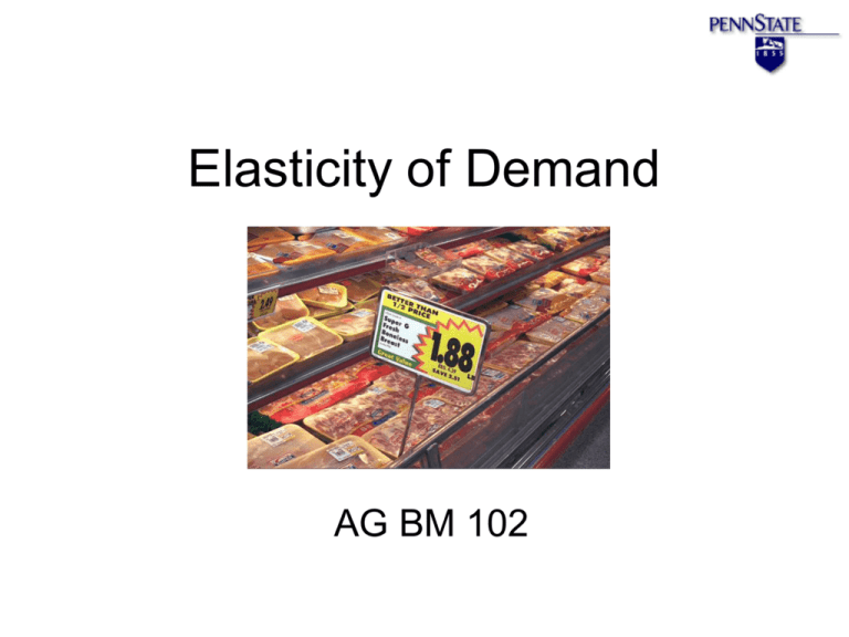
Elasticity of Demand
AG BM 102
Introduction
• Key issue: how responsive is the
consumption of a product to a change in
its price?
• The demand curve provides a quantitative
answer
• But the answer depends on units of
measurement
• Elasticity does not depend on units of
measurement!
Definition:
The own price elasticity of demand
- the percentage change in the
quantity demanded in response to
a one percent change in the price
of the product
An Example - Beef
Price/lb.
Price/lb.
$5.00
Quantity
lb./cap.
50
$3.75
Quantity
lb./cap.
75
$4.75
55
$3.50
80
$4.50
60
$3.25
85
$4.25
65
$3.00
90
$4.00
70
$2.75
95
Beef Demand
5
$/lb.
4
3
2
40
50
60
70
80
lbs./capita
90
100
Calculating the Equation for the
Demand Curve
• Take any two points, such as
$4.00 and 70 lb, and $3.00 and
90 lb.
• The equation for a straight line is
Q=a+bP
• In that equation a and b are
constants that together define a
specific line.
• You did this with x and y in
algebra
Q  a  bP
b  (Q1  Q2) / ( P1  P 2)
a  Q1  bP1
Q !  70lbs., P1  $4.00,
Q2  90lbs. and
b  (Q1  Q2) / ( P1  P 2)
b  (70  90) / (4  3)   20
a  Q1  bP1
a  70  ( 20) 4  150
Q  a  bP
Q  150  20 P
P 2  $3.00
Check to see if points
are on the line
Q = 150 – 20P
P = 4, Q = 150 - 20 (4) = 70
P = 5, Q = 150 - 20 (5) = 50
Formula for Demand Elasticity
  (Q  Q1) / (Q1) / ( P  P1) / ( P1)
2
2
Note: ε is the Greek letter epsilon
Elasticity at P=$4.00 and Q=70 lbs.
  (Q2  Q1) / (Q1) / ( P2  P1) / ( P1)
  (90  70) / (70) / (3  4) / (4)   114
.
Interpreting elasticity
• Inelastic
• Elastic
• Unitary elastic
0    1
 1    
  1
Inelastic demand means that the
quantity change is proportionately
less than the price change
Demand is not especially price
responsive – an example, the
demand for milk
Elastic demand means that the
quantity change is proportionately
more than the price change.
Demand is particularly price
responsive – an example, the
demand for lobster
Another view of the formula
Point elasticity
  (Q  Q1) / (Q1) / ( P  P1) / ( P1)
2
2
  (Q2  Q1) / ( P2  P1) *( P1) / (Q1)  b( P1 / Q1)
Note
• The units cancel out, so elasticity is not
dependent on the units used in the data
• For straight-line demand curves, the value
of the elasticity changes as you move
along the line
• The closer you are to the vertical axis the
more elastic is demand
• The closer to the horizontal axis the more
inelastic is demand
Elasticity at P=$5.00 and Q=50 lbs.
  b P / Q   20 (5 / 50)   2.0
Elasticity at P=$4.00 and Q=70 lbs.
  b P / Q   20 (4 / 70)   114
.
Some demand issues
• Is the demand for all food elastic or
inelastic?
• Is the demand for all meat elastic or
inelastic?
• Is the demand for beef elastic or inelastic?
• Is the demand for prime rib elastic or
inelastic?
Concluding comments
• Elasticity allows us to talk about demand
without worrying about the units of
measurement
• It makes discussion of demand curves
easier
• Makes analysis of changes in demand
easier