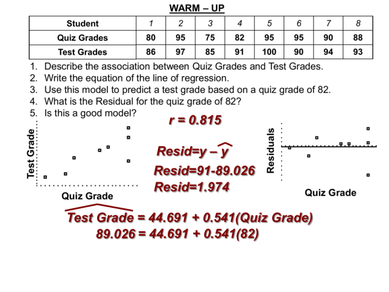
WARM – UP
1
2
3
4
5
6
7
8
Quiz Grades
80
95
75
82
95
95
90
88
Test Grades
86
97
85
91
100
90
94
93
Describe the association between Quiz Grades and Test Grades.
Write the equation of the line of regression.
Use this model to predict a test grade based on a quiz grade of 82.
What is the Residual for the quiz grade of 82?
Is this a good model?
Resid=y – y
Quiz Grade
Resid=91-89.026
Resid=1.974
Residuals
r = 0.815
Test Grade
1.
2.
3.
4.
5.
Student
Quiz Grade
Test Grade = 44.691 + 0.541(Quiz Grade)
89.026 = 44.691 + 0.541(82)
1 True Slope of the linear relationship.
H 0: β 1 = 0
H a: β 1 ≠ 0
A Linear Relationship
does NOT exist
A Linear Relationship
does exist
Regression Output Analysis
WARM – UP
The Statistics had an average of 81.2 with a standard deviation
of 4.5.
a.) What score represents the 90th percentiles?
x
x  81.2 x = 86.969
z
z = InvNorm(0.90) = 1.282 1.282 

4.5
b.) What is the probability that at least 3 out of 8 randomly
selected students scored in the top 10%.
P( x  3)  1  P( x  2)
 1  Binomialcdf (8, 0.10 , 2) = 0.0381
c.) Assuming a Normal Distribution, what is the probability that
a random sample of 3 students will have a mean score
of at least 85?
85  81.2
x 
)
P ( x  85) P( z 
z
4.5 / 3
 n
P( z  1.463)
Prob. = Normalcdf(1.463,∞) = 0.0718
WARM – UP
Many Economist believe that the down turn of the US
Economy is due to developments in the Housing Market. The
table below indicates random Medium home prices and the
Unemployment Rate at that time.
DATE
3/07
6/07
10/07 12/07
Housing $100K
263
236
234
Unemployment Rate
4.40
4.50
4.70
5/08
7/08
11/08
1/09
228
229
221
225
201
5.00
5.50
5.70
6.70
7.60
1. Describe the association between Housing values and
Unemployment.
2. Write the equation of the line of regression.
3. Use this model to predict unemployment if housing
reaches $180,000.
4. Is this a good model?
3/07
6/07
Housing $100K
263
236
234
Unemployment Rate
4.40
4.50
4.70
10/07 12/07
5/08
7/08
11/08
1/09
228
229
221
225
201
5.00
5.50
5.70
6.70
7.60
Describe the association between Housing values and Unemployment.
Write the equation of the line of regression.
Use this model to predict unemployment if housing reaches $180,000.
Is this a good model?
Residuals
Unemployment
1.
2.
3.
4.
DATE
Housing $100K
Housing $100K
Unemployment = 17.934 – 0.054(Housing $K)
8.197 = 17.934 – 0.054(180)
LINEAR REGRESSION t – TEST
b1  0
t
SE  b1 
P  Value  2  tcdf ( t , E 99, df n  2 )
# Hours of Study
.5
3
1.5
2
1.5
1
Test Grade
72
98
82
89
76
73
Does a significant relationship exist between number of
hours studying and test grades?
H :β =0
Grade  63.663  11.371(hours)
11.371  0
t
1.6803
0
1
Ha: β1 ≠ 0
SE  b1   1.6803
P  Value  2  tcdf ( 6.767 , E 99, 4)
 0.0025
Chapter 27 – INFERENCE FOR REGRESSION
– Spread around the line = se:
• The spread around the line is measured with
the standard deviation of the residuals se.
Chapter 27 – INFERENCE FOR REGRESSION
– Spread of the x values = sx:
• A large standard deviation of x provides a
more stable regression.
– Spread around the line = se
– Spread of the x values = sx
– Sample Size = n
SE  b1  
se
n  1  sx
SE(b1) is the Standard Error about the slope.
LINEAR REGRESSION t – TEST
Used to determine whether a significant relationship
exists between two quantitative variables.
t
x 
s /
n

b1  0
t
SE  b1 
β=0
β≠0
A Linear Relationship
does NOT exist
A Linear Relationship
does exist
WARM – UP
Many Economist believe that the current situation of the US Economy is
due to developments in the Housing Market. The table below indicates
random Medium home prices and the Unemployment Rate at that time.
DATE
3/07
6/07
10/07 12/07
Housing $100K
263
236
234
Unemployment Rate
4.40
4.50
4.70
5/08
7/08
11/08
1/09
228
229
221
225
201
5.00
5.50
5.70
6.70
7.60
Dependent Variable is: URate
R-squared = 68.1%
s = 0.69127 with 8 – 2 = 6 degrees of freedom
Variable Coefficient SE(Coeff) T-ratio P-Value
Intercept 17.93434
14.20411 1.6249 0.1386
Housing -0.05410
0.015115 -3.5792 0.0117
= b1
= SE(b1)
.05410  0
b1  0
t
t
 3.5792
0.015115
SE  b1 
P  Value  2  tcdf ( 3.5792 , E 99, 6)  0.0117
Chapter 27 – INFERENCE FOR REGRESSION
– Sample Size = n:
• Having a larger sample size, n, gives more
consistent estimates.