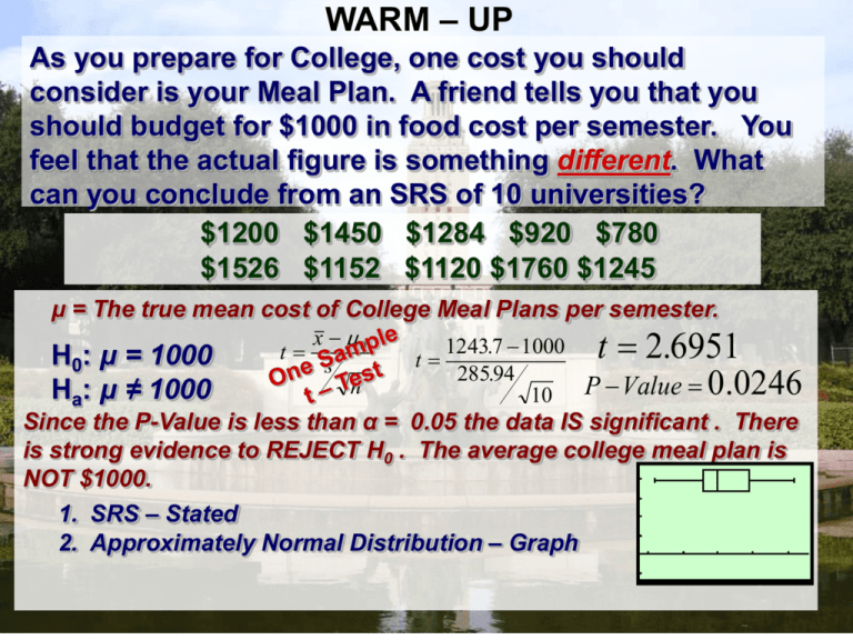
WARM – UP
As you prepare for College, one cost you should
consider is your Meal Plan. A friend tells you that you
should budget for $1000 in food cost per semester. You
feel that the actual figure is something different. What
can you conclude from an SRS of 10 universities?
$1200 $1450 $1284 $920 $780
$1526 $1152 $1120 $1760 $1245
μ = The true mean cost of College Meal Plans per semester.
x  0
1243.7  1000
H0: μ = 1000
Ha: μ ≠ 1000
t
t
s
n
285.94
10
t  2.6951
P  Value  0.0246
Since the P-Value is less than α = 0.05 the data IS significant . There
is strong evidence to REJECT H0 . The average college meal plan is
NOT $1000.
1. SRS – Stated
2. Approximately Normal Distribution – Graph
CHAPTER 25
MATCHED PAIRS t–TESTS
Objective: Use the One sample t procedures to interpret a
Matched Pairs t-test and be able to make inferences
about the differences in the two treatments which
share a common characteristic.
In a Matched Pairs design subjects are matched in
Homogeneous pairs or the same subject is used in both
treatments. A common type is a Before-and-After Design.
This leads to two Dependent data sets of which you
subtract.
The Matched Pairs t-Procedures
The Parameters and Statistics:
μd = the true mean difference in the two populations.
xd = the sample mean of all the differences of each
individual pairing.
sd = the sample standard deviation of all the differences
1. Confidence Interval:
sd
xd  t 
n
*
2. T-Test:
Precede with a ONE SAMPLE t-Test for the mean difference with
μd always equal to Zero.
H0: μd = 0
Ha: μd ≠, <, or > 0
xd  0
t
sd
n
P-VALUES
μd<0: tcdf(-E99, t, df)
μd>0: tcdf(t, E99, df)
μd≠0: 2·tcdf(|t|, E99, df)
EXAMPLE 1:
Many drivers of cars that can run on regular gas actually buy
premium in the belief that they will get better gas mileage. To
test this, 10 cars are randomly selected. Each car is run using
both regular and premium gas. The mileage is recorded. Is
there sufficient evidence at the 0.05 level to support the belief?
Car # Reg. Prem.
Prem.
–Reg.
1
16
19
3
2
20
22
2
3
21
24
3
4
22
24
2
5
23
25
2
6
22
25
3
7
27
26
-1
8
25
26
1
9
27
28
1
10
28
32
4
μd = The true mean DIFFERENCE in gas
mileage (Premium – Regular)
H0: μd = 0
Ha: μd > 0
t
xd  2 sd  1414
.
xd  0
sd
n
t
20
1414
.
10
t  4.4721 P  Value  0.0008
Since the P-Value < α = 0.05 - REJECT H0
STRONG evidence that Premium Gas does
improve gas mileage.
1. SRS – Stated
2. Approximately Normal Distribution – Graph
EXAMPLE 2:
“Freshman – 15” Many people believe that students gain a
significant amount of weight their freshman year of college. Is
there enough evidence at the 5% level to support that there is
a weight increase? Use the weights of 6 randomly chosen
students. Student weights were measure at the beginning and
at the end of the fall semester.
Begin
End
End–
Begin
1
171
168
-3
2
110
111
1
3
134
136
2
4
115
119
4
5
150
155
5
6
104
106
2
μd = The true mean DIFFERENCE in Weight
in pounds (End of Semester – Beginning)
1.833  0
xd   d
H :μ =0
0
d
t
sd
t
Ha: μd > 0
n
xd  1.833 sd  2.787
t  1.611
2.787
6
P  Value  0.0840
Since the P-Value is NOT less than α = 0.05
Fail to REJECT H0 . The belief that Freshman
experience weight increase `is not supported.
1. SRS – Stated
2. Approximately Normal Distribution – Graph
EXAMPLE 3:
The maker of a new tire claims that his Tires are superior in all
road conditions. He claims that with his tires there is no
difference in stopping distance between dry or wet pavement.
To test this you select an SRS of 9 cars and at 60 mph you
slam on the breaks. Estimate the Mean difference in stopping
distance in feet with a 90% Confidence Interval.
μd= The true mean DIFFERENCE in stopping
distance in feet (Wet – Dry Pavement)
s
Matched Pairs
xd  t *  d
n
1-Sample
xd  55 sd  10.210
t – Interval
F I
H K
55  1.86  10.210 
9

55  7.848
We are 90% Confident that the True mean
difference in stopping distance in feet
between Wet Pavement – Dry Pavement is
between 48.671 ft and 61.329 ft.
1. SRS – Stated
2. Approximately Normal Distribution – Graph
Car # Wet
Dry
Wet –
Dry
1
201
150
51
2
220
147
73
3
192
136
56
4
182
130
52
5
173
134
39
6
202
134
68
7
180
128
52
8
192
136
56
9
206
158
48
Chips Ahoy used to advertise “1000 Chips in Every Bag!”
1. How would YOU do a significance test to test this?
2. What issues do you think would arise and how would
you over come them?
1000 Chips in
Every Bag!
Chips Ahoy used to advertise “1000 Chips in Every Bag!”
With 38 cookies in each bag, the true mean number of
chips in each cookie should be 26.3 chips per cookie.
Because there was a suspicion of LESS than 26.3 chip per
cookie the company disregarded the ad. Test this claim by
crumbling cookies and counting the number of chips in
each.
a.) Is there evidence to support the company’s decision.
Gather evidence and Conduct a Significance test.
b.) Estimate the true # of chips in the bag by finding a
95% Confidence Interval for the true # of chips per
cookie and then multiply it by 38.
c.) Eat your evidence.
1000 Chips in
Every Bag!