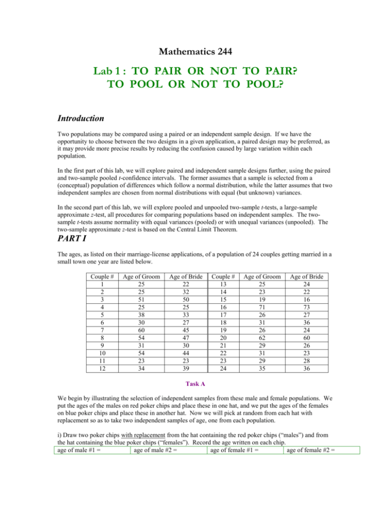
Mathematics 244
Lab 1 : TO PAIR OR NOT TO PAIR?
TO POOL OR NOT TO POOL?
Introduction
Two populations may be compared using a paired or an independent sample design. If we have the
opportunity to choose between the two designs in a given application, a paired design may be preferred, as
it may provide more precise results by reducing the confusion caused by large variation within each
population.
In the first part of this lab, we will explore paired and independent sample designs further, using the paired
and two-sample pooled t-confidence intervals. The former assumes that a sample is selected from a
(conceptual) population of differences which follow a normal distribution, while the latter assumes that two
independent samples are chosen from normal distributions with equal (but unknown) variances.
In the second part of this lab, we will explore pooled and unpooled two-sample t-tests, a large-sample
approximate z-test, all procedures for comparing populations based on independent samples. The twosample t-tests assume normality with equal variances (pooled) or with unequal variances (unpooled). The
two-sample approximate z-test is based on the Central Limit Theorem.
PART I
The ages, as listed on their marriage-license applications, of a population of 24 couples getting married in a
small town one year are listed below.
Couple #
1
2
3
4
5
6
7
8
9
10
11
12
Age of Groom
25
25
51
25
38
30
60
54
31
54
23
34
Age of Bride
22
32
50
25
33
27
45
47
30
44
23
39
Couple #
13
14
15
16
17
18
19
20
21
22
23
24
Age of Groom
25
23
19
71
26
31
26
62
29
31
29
35
Age of Bride
24
22
16
73
27
36
24
60
26
23
28
36
Task A
We begin by illustrating the selection of independent samples from these male and female populations. We
put the ages of the males on red poker chips and place these in one hat, and we put the ages of the females
on blue poker chips and place these in another hat. Now we will pick at random from each hat with
replacement so as to take two independent samples of age, one from each population.
i) Draw two poker chips with replacement from the hat containing the red poker chips (“males”) and from
the hat containing the blue poker chips (“females”). Record the age written on each chip.
age of male #1 =
age of male #2 =
age of female #1 =
age of female #2 =
ii) Report your results to the Lab Instructor, who will display the collected results. Type the collected
values into MINITAB.
iii) What is the sample mean age of males (X)? What is the sample mean age of females (Y)? What is the
difference of these two sample means?
x =
xy =
y =
iv) What does the difference of the sample means estimate?
v) What is the sample variance of the age of males (X)? What is the sample variance of the age of females
(Y)? What is the pooled variance
s 2p of the ages for these two samples? What is the pooled standard
error SEp of the ages?
Recall that the formula for
s is s 
2
p
2
p
(n x  1) s x2  (n y  1) s y2
nx  n y  2
and that the formula for SEp is
 1
1 
SE p  s 2p    .
n

 x ny 
The MINITAB commands to calculate
s 2p and SEp are as follows, for independent samples stored in
columns c1 and c2:
2
let k1 = stdev(c1)**2
 sx
let k2 = stdev(c2)**2

let k3 = n(c1)
let k4 = n(c2)
s y2
 nx
 ny
let k5 = ((k3–1)*k1 + (k4–1)*k2) / (k3+k4–2)
let k6 = sqrt(k5*(1/k3 + 1/k4))

s 2p
 SEp
s x2 =
s y2 =
s 2p =
SEp =
vi) If the two populations were normal with equal variances, what would be the margin of error of a 90%
confidence interval for  X  Y ?
Task B
Now we consider a paired-sample design, where couples are sampled instead of individuals. We place
poker chips stuck together, with the ages of the male (red) and the female (blue) for that couple, into one
hat. Now we will pick pairs of chips from each hat with replacement, so as to take one sample of paired
observations.
i) Draw two poker-chip pairs with replacement from the hat containing the poker-chip “couples”. Again
the males are red and the females are blue. Record the ages of both “partners” in the “couple.” Calculate
the difference in their ages.
age of male in couple #1 =
age of male in couple #2 =
age of female in couple #1 =
age of female in couple #2 =
difference in age #1 =
difference in age #2 =
ii) Report your results to the Lab Instructor, who will display the collected results. Type the collected
values into MINITAB.
iii) What is the mean of the age differences in the sample?
d =
iv) What does this mean difference estimate?
2
v) What is the sample variance s d of the age differences in the sample? What is the standard error SE of
the age differences? How does the standard error of the age difference compare to the pooled standard
error SEp of the ages obtained in Task A?
SE =
s2 =
d
comparison of SE to SEp:
vi) If the population of differences were normal, then what would be the margin of error of a 90%
confidence interval for  d ?
vii) Which procedure is more accurate for estimating the mean age difference between males and females
at marriage? Explain.
Task C
i) If X and Y are correlated, then V(X–Y) = V(X) + V(Y) – 2Cov(X,Y) =  X
2
where
 XY  corr ( X , Y ) 
Cov( X , Y )
  Y2  2  XY  X  Y ,
. Let’s verify this relationship by calculating the sample
V ( X )V (Y )
variances of the males and females in the couples and sample correlation coefficient (corr cX cY) to
estimate V(X–Y) =
 d2 . The population data are in the first three columns of the MINITAB worksheet
lab7dat.mtw. Although we have the entire population, MINITAB’s commands calculate sample statistics,
so we’re only estimating the population variances and correlation, which we will label
̂ XY , ˆ X2 , ˆ Y2 ,
2
and ˆ d .
Copy your commands and output here. Be sure to annotate your output to identify all quantities. Compare
2
2
the estimate ˆ d to s d .
̂ XY =
ˆ X2 =
s d2 =
comparison:
ii) What is Cov(X,Y) when X and Y are independent?
ˆ Y2 =
ˆ d2 =
iii) When the covariance is positive, for which sampling procedure is the variance of the difference
smaller?
Conclusion
If we were to examine the ages at marriage in a population of married women, we would find considerable
variation. Similarly, we would see considerable variability in marriage-age if we were to examine a
population of married men. The difference in marriage-ages between men and women would reflect the
variability in the independent populations. But when we examine the difference in ages at marriage in a
population of men and women as couples, we find there is far less variability.
PART II
You may have wandered through shopping malls a few years ago and seen crowds of people staring
intently at pictures for sale. You probably glanced at such pictures and noticed that they appeared to
contain only dots.
Random dot stereograms are pairs of images which appear to be composed entirely of random dots but
which are actually constructed so that a 3D image will be seen, if the images are viewed with a stereo
viewer, causing the separate images to fuse. Another way to fuse the images is to fixate on a point between
them and defocus the eyes, but this technique takes some effort and practice1 (and lots of free time!).
J. P. Frisby and J. L. Clatworthy2 performed an experiment to determine whether knowledge of the form of
the embedded image (of a spiral staircase) affected the time required for subjects to fuse the images. One
group of subjects (group NV) received either no information or just verbal information about the shape of
the embedded object. A second group (group VV) received both verbal information and visual information
(e.g., a drawing of the object).1
Columns C5 and C6 of the MINITAB worksheet lab1dat.mtw contain the time to produce a fused image
of the random dot stereogram for the two treatment groups for this experiment. 3
Task A
We want to test H0: NV – VV = 0, Ha: NV – VV  0 at the .05 level of significance. In this part of the lab,
we will perform several tests of hypothesis for the difference of location of two independent populations,
without considering yet whether these tests are totally appropriate for this data.
i) Perform the two-sample pooled t-test and generate a 95% confidence interval for NV – VV (commands
in appendix). Copy your commands and results here.
ii) Perform the two-sample unpooled t-test and generate a 95% confidence interval for NV – VV
(commands in appendix). Copy your commands and results here.
iii) Perform the Mann-Whitney-Wilcoxon test and generate a 95% confidence interval for MNV – MVV
(commands in appendix). Copy your commands and results here.
iv) Perform the two-sample approximate z-test and compute an approximate 95% confidence interval for
NV – VV. The procedures are as follows:
a) Calculate
z0 
( X NV  X VV )  0
, where SE 
SE
2
s NV
s2
 VV .
n NV nVV
b) Reject H0 if |z0|  z/2.
c) Calculate the confidence interval: ( X NV  X VV )  z / 2  SE .
1
Description from the StatLib Data and Stories Library at
http://lib.stat.cmu.edu/DASL/Stories/FusionTime.html .
2
Frisby, J.P., and Clatworthy, J.L. 1975. Learning to see complex random-dot stereograms. Perception 4:
173-178.
3
Data obtained from StatLib Data and Stories Library at
http://lib.stat.cmu.edu/DASL/Datafiles/FusionTime.html . Source: Cleveland, W.S. 1993. Visualizing
Data. Hobart Press (Summit, NJ).
Note that z0 is the same as t0 calculated for the unpooled t-test. The difference in the tests is in the use of
the critical value z/2 rather than t/2.
Copy your commands and results here. Be sure to label each quantity.
v) Summarize the results of the tests and confidence intervals:
Test
Decision
(a) two-sample pooled t-test
(b) two-sample unpooled t-test
(c) Mann-Whitney-Wilcoxon test
(d) two-sample approximate z-test
Confidence Interval
vi) Should we pick the result we like from the above, or should we try to see which result is valid?
Task B
Now we will determine which test would have been the appropriate test to use, based on whether the
underlying assumptions for each test are reasonable, given the characteristics of the samples.
i) Generate descriptive statistics for the data.
ii) Perform the Ryan-Joiner normal-scores test for non-normality on the data (commands in appendix).
NV
VV
iii) Generate stem-and-leaf plots of the data.
iv) Generate simultaneous boxplots of the data.
v) Based on the descriptive statistics, non-normality test results, stem-and-leaf plots, and boxplots,
determine which of procedures (a), (b), or (c) is appropriate to use.
Conclusion
Although we technically could perform the large-sample test in this case, it is only approximate, so that
result (d) is less credible than that of an exact test. The exact test is the appropriate test to use when it is
reasonable to do so.
Appendix: MINITAB commands
The procedures for performing paired t-tests and calculating t-confidence intervals are as follows:
Paired t-Test
TYPING COMMANDS
USING THE MOUSE
MTB > ttest c3 ;
Stat Basic Statistics  1-Sample t...
SUBC> alte direction .
Type the identity of the column of sample differences
in the Variables: box.
where direction is –1 for a left-tailed
test, 1 for a right-tailed test, or 0 for Select Test mean: and type the value of the
a two-tailed test
hypothesized mean difference in the box.
Note: “alte” is an abbreviation for
“alternative”
Select the appropriate Alternative: less than for a
left-tailed test, greater than for a right-tailed test,
or not equal for a two-tailed test
Click OK.
Paired t-CI
TYPING COMMANDS
USING THE MOUSE
MTB > tint conf_level c3
Stat Basic Statistics  1-Sample t...
where conf_level is the desired level
of confidence, in percent
Type the identity of the column of sample differences
in the Variables: box.
Select Confidence interval and type the desired
confidence Level, in percent, in the box.
Click OK.
The procedure for performing the Ryan-Joiner Test for non-normality is as follows:
USING THE MOUSE
Stat Basic Statistics  Normality Test...
Type the identity of the sample column in the Variable: box.
Select the Ryan-Joiner test for non-normality.
Click OK.
The procedures for performing two-sample t-tests are as follows:
Pooled 2-Sample t-Test — data in 2 columns
TYPING COMMANDS
USING THE MOUSE
MTB > twos conf_level c1 c2 ;
Stat Basic Statistics  2-Sample t...
SUBC> alte direction ;
Select Samples in different columns and type the
identities of the First and Second sample columns
in the corresponding boxes.
SUBC> pool .
where direction is –1 for a left-tailed
test, 1 for a right-tailed test, or 0 for Select the appropriate Alternative: less than for a
left-tailed test, greater than for a right-tailed test,
a two-tailed test
or not equal for a two-tailed test
and conf_level is the desired level of
Select Assume equal variances.
confidence, in percent
Specify the desired Confidence level in percent.
Note: “twos” is an abbreviation for
“twosample” and “alte” is an
abbreviation for “alternative”
Click OK.
Unpooled 2-Sample t-Test — data in 2 columns
TYPING COMMANDS
USING THE MOUSE
MTB > twos conf_level c1 c2 ;
Same as above, except
SUBC> alte direction .
Ensure that Assume equal variances is NOT checked.
The procedure for performing the Mann-Whitney-Wilcoxon test is as follows (data MUST be in 2
columns):
TYPING COMMANDS
USING THE MOUSE
MTB > mann conf_level c1 c2 ;
Stat Nonparametrics  Mann-Whitney...
SUBC> alte direction .
Type the identities of the First and Second sample
columns in the corresponding boxes.
Note: “mann” is an abbreviation for
“Mann-Whitney”
Specify the desired Confidence level in percent.
Select the appropriate Alternative.
Click OK.