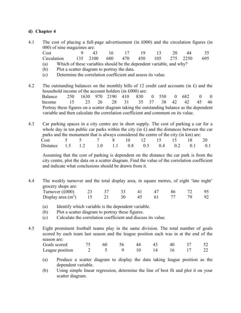
d) Chapter 4
4.1
The cost of placing a full-page advertisement (in £000) and the circulation figures (in
000) of nine magazines are:
Cost
9
43
16
17
19
13
20
44
35
Circulation
135 2100
680
470
450
105
275 2250
695
(a)
Which of these variables should be the dependent variable, and why?
(b)
Plot a scatter diagram to portray the data.
(c)
Determine the correlation coefficient and assess its value.
4.2
The outstanding balances on the monthly bills of 12 credit card accounts (in £) and the
household income of the account holders (in £000) are:
Balance
250 1630 970 2190 410
830
0 550
0 682
0
0
Income
15
23
26
28
31
35 37
38 42
42
45 46
Portray these figures on a scatter diagram taking the outstanding balance as the dependent
variable and then calculate the correlation coefficient and comment on its value.
4.3
Car parking spaces in a city centre are in short supply. The cost of parking a car for a
whole day in ten public car parks within the city (in £) and the distances between the car
parks and the monument that is always considered the centre of the city (in km) are:
Cost
5
5
7
8
10
12
15
15
18
20
Distance
1.5
1.2
1.0
1.1
0.8
0.5
0.4
0.2
0.1
0.1
Assuming that the cost of parking is dependent on the distance the car park is from the
city centre, plot the data on a scatter diagram. Find the value of the correlation coefficient
and indicate what conclusions should be drawn from it.
4.4
The weekly turnover and the total display area, in square metres, of eight ‘late night’
grocery shops are:
Turnover (£000)
23
37
33
41
47
86
72
95
Display area (m2)
15
21
30
45
61
77
79
92
(a)
(b)
(c)
4.5
Identify which variable is the dependent variable.
Plot a scatter diagram to portray these figures.
Calculate the correlation coefficient and discuss its value.
Eight prominent football teams play in the same division. The total number of goals
scored by each team last season and the league position each was in at the end of the
season are:
Goals scored
75
60
56
44
43
40
37
52
League position
2
5
9
10
14
16
17
22
(a)
(b)
Produce a scatter diagram to display the data taking league position as the
dependent variable.
Using simple linear regression, determine the line of best fit and plot it on your
scatter diagram.
(c)
4.6
Predict the final position of a team that scored 50 goals using your regression
equation.
In a survey of commuting patterns ten respondents say that they cycle to work. The
distances they travel (in miles) and the mean journey times (in minutes) they report are:
Distance
2
2
3
4
5
6
7
8
8
10
Mean journey time 10
15
15
20
25
25
30
40
45
50
(a)
(b)
(c)
4.7
Portray the data on a scatter diagram.
Calculate the slope and intercept of the line of best fit using simple linear
regression analysis.
Plot the line of best fit and use it to estimate the time that a journey of 9 miles
would take.
The classified advertisement columns of a local paper contain details of twelve used cars
of a particular make and model. The prices of these cars (in £000) and the numbers of
miles they have travelled (in 000) are:
Price
6.8 6.2 5.7 4.7 6.0 5.9 7.0 4.5 5.0 3.0 3.8 3.5
Mileage 9
13
11
33
14
11
3
19
22
35
40
44
(a)
(b)
(c)
Present these figures in the form of a scatter diagram.
Find the least squares line of best fit and plot it on your scatter diagram.
Predict the price of a car of this type that has travelled 25 000 miles.
4.8
A cab driver pays for fuel, vehicle servicing and maintenance every 3 months, and an
annual operating licence. The prices of these in 2009 and in 2005, together with the
quantity of each that was purchased during 2005 are:
Item
Price in 2009 (£)
Price in 2005 (£)
Quantity bought in 2005
Fuel (litre)
1.10
0.78
4100
Servicing
115.00
83.00
4
Licence
750.00
500.00
1
(a)
(b)
(c)
4.9
Calculate the weighted aggregate price index for the prices in 2009 based on the
prices in 2005 using the Laspeyre method.
In 2009 the driver purchased 4000 litres of fuel, had the vehicle serviced four
times and bought the annual licence. Use these figures to calculate the weighted
aggregate price index for 2009 with 2005 as the base year using the Paasche
method.
Compare the results to (a) and (b) and advise the driver, who is not good at
keeping records, which method of assessing overall changes in costs would be
more suitable.
A textile manufacturer makes casual jackets. The company buys lining fabric, interfacing
fabric and outer fabric. These fabrics are cut and machined to make the garments. The
prices per metre of these materials in 2007, 2008 and 2009 were:
Year
Fabric
2007
2008
2009
Lining
£2.20
£2.30
£2.35
Interfacing
Outer
£0.92
£6.50
£0.95
£7.25
£1.00
£7.95
In 2007 the company purchased 2500 metres of lining fabric, 400 metres of interfacing
fabric, and 2750 metres of outer fabric. In 2008 these quantities were 2800, 500, and
3200 respectively. In 2009 they were 3000, 500, and 5000 respectively.
(a)
Calculate Laspeyre price indices for 2008 and 2009 using 2007 as the base period.
(b)
Calculate Paasche price indices for 2008 and 2009 using 2007 as the base period.
(c)
Compare your answers to (a) and (b) and account for any differences between the
values of the price indices.
4.10
A confectioner buys cocoa, cocoa butter, sugar, and milk solids. The prices per kilogram
of these ingredients in 2003, 2006, and 2009 were:
Year
Ingredient
2003
2006
2009
Cocoa
£1.50
£1.45
£1.70
Cocoa butter
£1.30
£1.95
£2.05
Sugar
£0.45
£0.50
£0.55
Milk solids
£0.35
£0.62
£0.68
The quantities that were purchased in 2003 were 7500 kg of cocoa, 4200 kg, of cocoa
butter, 12000 kg of sugar, and 5700 kg of milk solids. The purchased amounts of these
items in 2006 were 8000 kg, 4000 kg, 13000 kg, and 6000 kg respectively. In 2009 they
were 8800 kg, 3100 kg, 15000 kg, and 4500 kg respectively.
(a)
Compile Laspeyre price indices for 2006 and 2009 using 2003 as the base year.
(b)
Compile Paasche price indices for 2006 and 2009 using 2003 as the base year.
(c)
Compare your results for (a) and (b) suggesting reasons for any differences
between them.
4.11
The turnover figures provided in the annual accounts of a large retail grocer over the six
years from 2003 to 2008 were:
Year
2003
2004
2005
2006
2007
2008
Turnover (£m)
7022
7101
7350
7844
8249
8598
The values of the Retail Price Index (RPI) for this period were:
Year
2003
2004
2005
2006
RPI
181.3
186.7
192.0
198.1
2007
206.6
2008
215.3
Use the RPI values to deflate the turnover figures so that they are all expressed in 2003
pounds.
4.12
An enthusiast paid £5000 for a classic car in 2000. Since that time the car has been kept
carefully and been valued every two years. The valuations were:
Year
2002
2004
2006
2008
Valuation (£)
5200
5500
6200
6000
The values of the Retail Price Index (RPI) for these years were:
Year
2002
2004
2006
2008
RPI
176.2
186.7
198.1
215.3
Use the values of the RPI to adjust the valuations of the car so that they are all expressed
in 2000 pounds. The value of the RPI in 2000 was 170.3.
4.13
A body-piercing and tattoo studio is open each day of the week except Sundays and
Mondays. The number of customers visiting the studio per day over a period of three
weeks is:
Week
Tuesday
Wednesday
Thursday
Friday
Saturday
1
5
8
9
18
34
2
4
8
11
22
39
3
7
9
14
21
42
(a)
(b)
(c)
(d)
(e)
4.14
The amounts of gas (in thousands of gigawatt hours) sold to domestic consumers by a
regional energy company over three years were:
Quarter
Year
Winter
Spring
Summer
Autumn
1
28
12
7
23
2
27
14
7
24
3
28
13
6
24
(a)
(b)
(c)
(d)
4.15
Plot the time series.
Calculate five-point moving averages for the series.
Estimate daily components for the series.
Produce estimates for the values of the trend in week 4 using regression analysis.
Compile forecasts for the number of visitors the studio should expect on each day
in week 4.
Produce a graph to represent the figures.
Determine centred four-point moving averages for the time series.
Find the seasonal component for each quarter.
Compile forecasts for the four quarters of year 4.
A High Street chemist sells travel first aid packs. The numbers of these sold over three
years were:
Quarter
Year
Winter
Spring
Summer
Autumn
1
11
37
61
18
2
13
49
58
16
3
16
53
66
18
(a)
(b)
(c)
(d)
Plot a graph to portray the data.
Calculate centred four-point moving averages for the time series.
Determine the seasonal component for each quarter.
Compile forecasts for the four quarters of the fourth year.
4.16
Select the appropriate definition
right hand side.
(a)
A regression equation
(b)
A correlation coefficient
(c)
A moving average
(d)
An inverse relationship
(e)
A predictor
(f)
A response
(g)
A trend
(h)
A weighted price index
for each term on the left-hand side from the list on the
(i)
(ii)
(iii)
(iv)
(v)
(vi)
(vii)
(viii)
is another name for the dependent variable, Y
is an underlying movement in a time series
measures price changes over time
is another name for the independent variable, X
is a mean of a sequence of time series values
measures association between two variables
is when Y goes down as X goes up
represents the line of best fit