7 Sorting
Sorting is a fundamental task that can be a deciding factor in the overall performance of
the system. In this section, we will consider several algorithms that can sort data. The
performance of these algorithms can vary widely. Some algorithms are complex but
work fast. Some are slow but very easy to write.
7.1
Simple Sorts
There are several sorts that are relatively easy to code. These are considered to be
"simple sorts" and generally have bad run time O(n2).
7.1.1 Bubble Sort
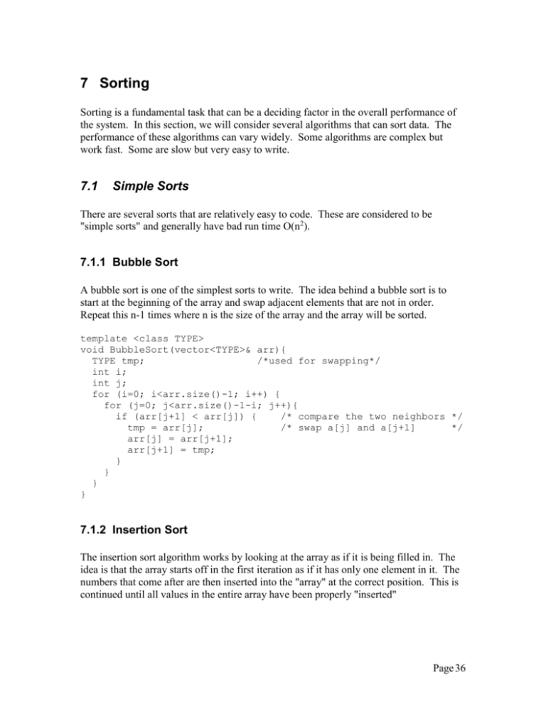
A bubble sort is one of the simplest sorts to write. The idea behind a bubble sort is to
start at the beginning of the array and swap adjacent elements that are not in order.
Repeat this n-1 times where n is the size of the array and the array will be sorted.
template <class TYPE>
void BubbleSort(vector<TYPE>& arr){
TYPE tmp;
/*used for swapping*/
int i;
int j;
for (i=0; i<arr.size()-1; i++) {
for (j=0; j<arr.size()-1-i; j++){
if (arr[j+1] < arr[j]) {
/* compare the two neighbors */
tmp = arr[j];
/* swap a[j] and a[j+1]
*/
arr[j] = arr[j+1];
arr[j+1] = tmp;
}
}
}
}
7.1.2 Insertion Sort
The insertion sort algorithm works by looking at the array as if it is being filled in. The
idea is that the array starts off in the first iteration as if it has only one element in it. The
numbers that come after are then inserted into the "array" at the correct position. This is
continued until all values in the entire array have been properly "inserted"
Page 36
template <class TYPE>
void InsertionSort(vector<TYPE>& arr){
TYPE curr;
int i, j;
for(i=1;i<arr.size();i++){
curr=arr[i];
for(j=i;j>0 && arr[j-1] > curr;j--){
arr[j]=arr[j-1];
}
arr[j]=curr;
}
}
7.2
Mergesort
The idea of a merge sort is this. If you have 2 arrays that are already sorted, then you can
"merge" them into a single sorted array by choosing to add the smaller of the "next" item
between the two arrays.
3
5
6
9
1
2
7
8
1 < 3 so copy 1 into new array. Advance pointer on that array.
3
5
6
9
1
2
7
8
1
2 < 3 so copy 2 into new array and advance appropriate pointer
3
5
6
9
1
2
7
8
1
2
3 < 7 so copy 3 into new array and advance appropriate pointer
3
5
6
9
1
2
7
8
1
2
3
5 < 7 so copy 5 into new array and advance appropriate pointer
Page 37
3
5
6
9
1
2
7
8
1
2
3
5
6 < 7 so copy 6 into new array and advance appropriate pointer
3
5
6
9
1
2
7
8
1
2
3
5
6
5
6
7
5
6
7
7 < 9 so copy 7 into new array and advance appropriate pointer
3
5
6
9
1
2
7
8
1
2
3
8 < 9 so copy 8 into new array and advance appropriate pointer
3
5
6
9
1
2
7
8
1
2
3
8
All data from second array has been copied in so copy in last element of first array
3
5
6
9
1
2
7
8
1
2
3
5
6
7
8
9
The MergeSort function can be written recursively then in the following manner:
template <class TYPE>
void MergeSort(vector<TYPE>& arr, vector<TYPE>& tmp, int start,
int end){
if (start<end){
int mid=(start+end)/2;
MergeSort(arr,tmp,start,mid);
MergeSort(arr,tmp,mid+1,end);
Merge(arr,tmp,start,mid+1,end);
}
}
Page 38
/*This function merges the two halves of the array arr into tmp
and then copies it back into arr*/
template <class TYPE>
void Merge(vector<TYPE>& arr, vector<TYPE>& tmp, int start,
int start2, int end){
int aptr=start;
int bptr=start2;
int i=start;
while(aptr<start2 && bptr <= end){
if(arr[aptr]<arr[bptr])
tmp[i++]=arr[aptr++];
else
tmp[i++]=arr[bptr++];
}
while(aptr<start2){
tmp[i++]=arr[aptr++];
}
while(bptr<=end){
tmp[i++]=arr[bptr++];
}
for(i=start;i<=end;i++){
arr[i]=tmp[i];
}
}
template <class TYPE>
void MergeSort(vector<TYPE>& arr){
vector<TYPE> tmp(arr.size());
MergeSort(arr,tmp,0,arr.size()-1);
}
Merge Sort has an average and worst case run time of O(n log n). However, there is one
major drawback to this algorithm. This function requires the use of a temporary array.
This array means that you will have to use twice as much memory to do the sorting.
Furthermore, after each merge, the temporary array is copied back into the original array.
This also takes time.
The merge sort algorithm could also be written non-recursively quite easily. Observe the
indexes used to call MergeSort each time. Instead of using recursion, we could simply
start from the bottom and work our way up, merging as we go.
0 to 7
0 to 3
0 to 1
4 to 7
2 to 3
4 to 5
6 to 7
Page 39
7.3
Quick Sort
This sort is fast and does not have the extra memory requirements of MergeSort. On
average its run time is O(n log n) but it does have a worst case run time of O(n2)
QuickSort works like this:
1.
2.
3.
4.
5.
6.
7.
8.
Pick a value from the array as the pivot
Let i=front, j= back
advance i until you find a value arr[i] > pivot
move j towards front of array until arr[j] < pivot
swap these arr[i] and arr[j].
repeat step 3 to 5 until i and j meet
The meeting point is used to break the array up into two pieces
QuickSort these two new arrays
A simple version of the algorithm can be written as:
template <class TYPE>
void QuickSort(vector<TYPE>& arr, int left, int right){
if(right-left <=3){
InsertionSort(arr,left,right);
}
else{
int pivotpt=right;
int i=left;
int j=right-1;
TYPE pivot=arr[pivotpt];
while(i<j){
while(arr[i]<pivot) i++;
while(arr[j]>pivot) j--;
if(i<j)
swap(arr[i++],arr[j--]);
}
swap(arr[i],arr[pivotpt]);
QuickSort(arr,left,i-1);
QuickSort(arr,i+1,right);
}
}
template <class TYPE>
void QuickSort(vector<TYPE>& arr){
QuickSort(arr,0,arr.size()-1);
}
The idea of a quicksort is that with each call, the quicksort algorithm would break the
vector up into two parts. The best thing that can happen is that each time we get pieces
that are of equal size (ie we get two pieces that is half the size of the original vector). As
Page 40
you will recall from binary search, you can only half something log n times (where n is
the size of the vector) before you get a vector of size 0. Thus, for the best possible case,
the runtime is O(n log n).
The worst thing that can happen for the quicksort algorithm is to choose a pivot such that
we end up getting a pivot point that breaks up the vector into an empty vector and a
vector containing everything else every single time. If you do this, you will end up with
not reducing the size of the vector by much (just one for the pivot) and thus, your work
will be almost as much as it was to begin with. The worst case run time is O(n2)
The average runtime for quicksort is also O(n log n).
7.3.1 Median of Three partitioning
The algorithm that is shown above chooses the last element in the vector as the pivot.
This was done for simplicity but is actually not very good. If the elements are random,
then using the end of the array is not bad. However, if the data is nearly sorted to begin
with then picking the end point could very well mean picking the biggest value. This
would create the worst case scenario where one vector was empty and the other contained
everything else.
Recall that the best possible scenario occurs when we break down the list into two pieces
of the same size. To do this, our pivot must be the median value. The median is the
number where half of the other numbers are below it and half the other numbers are
above it. Thus, if our pivot was the median of the list each and every time, we would end
up with the best case scenario. However, finding the median is not an easy problem to
solve quickly so instead of trying to find the exact median, one strategy is to choose the
median of three values in the vector (use the three values like a sampling of the
population. Like polling!) This can be done by looking at the first, last and middle
element. From here choose the median value of the three as the pivot.
7.4
Heap Sort
Heap Sort is a sort based on the building and destroying of a binary heap. The binary
heap is an implementation of a priority Queue. Normally, when you have a Queue, the
first value in is the first value out. However with a priority Queue the value that comes
out of the Queue next depends on the priority of that value.
Basic operations on the binary Heap include:
 Insert - add an item to the binary heap
 Delete_Min - removes the smallest value in the binary heap.
The idea for the Heap sort is this: put every value in the array into the binary heap, then
repeated call Delete_Min to remove the smallest value and put it back into the array.
Page 41
7.4.1 Definitions
Binary Heap - A binary heap is a complete binary tree where the heap order property is
always maintained.
Binary Tree - A binary tree is either
a) empty (no nodes), or
b) contains a root node with two children which are both binary trees.
Example:
Complete Binary Tree - A binary tree where there are no missing nodes in all but the
bottom level. At the bottom level the missing nodes must be to the right of all other
nodes.
Examples (complete binary trees):
Not complete binary trees:
Page 42
Heap Order Property: The values in the children of each node must be bigger than that
in the node.
Example:
3
10
22
13
15
12
16
39
29
17
7.4.2 Insert
Insertion into a heap must maintain both the complete binary tree structure and the heap
order property. To do this what we do is the following.
We know that in order to maintain the complete binary tree structure, we must add a node
to the first open spot at the bottom level. So we begin by adding a node without data
there. After that what we do is we see if inserting our new value will violate the heap
property. If it doesn't put it in and we are done. Otherwise, we move the value from the
parent of the empty node down , thus creating an empty node where the parent use to be.
We again check to see if inserting the value violates the heap order property. If not, we
add it in. Otherwise repeat the process until we are able to add the value. This process of
moving the empty node towards the root is called percolate up
Example: Insert into a heap the following values in order: 10,6,20,5, 16, 17, 13,2
Insert 10:
10
Insert 6:
10
6
10
10
Page 43
Insert 20
6
6
10
10
20
Insert 5
6
6
10
20
20
10
5
6
20
10
6
20
10
Insert 16
5
6
10
5
20
6
10
20
16
Page 44
Insert 17:
5
5
6
10
20
6
16
10
20
16
5
6
17
10
20
16
Insert 13
5
5
6
10
17
16
6
20
10
16
20
17
5
6
10
13
16
20
17
Page 45
Insert 2:
5
5
6
16
10
6
13
16
17
20
13
17
20
10
5
5
13
16
6
6
17
20
10
13
16
20
17
10
2
5
6
13
16
20
17
10
Page 46
7.4.3 Delete_Min
This is the process of removing the smallest value from the binary heap. The way that
the Heap is set up, the smallest value is at the root. Finding the value is simple but the
removal process must ensure that both the complete binary tree structure along with the
heap order property is maintained. In order for the binary tree property to be maintained
we will be removing the right most node at the bottom level. The empty spot that had
been created by the removal of the value at root must be filled and the value that had been
in the rightmost node must go back into the heap. The process is this:



If the value could be placed into the empty spot without violating the Heap Order
Property, put it in and we are done
otherwise move the smaller of the nodes children up (the empty spot moves
down).
Repeat process
The process of moving the empty spot down the heap is called percolate down
Diagram of this is on the next page
Page 47
Example: Delete_Min on following heap
2
5
16
6
5
13
17
20
13
16
6
17
20
we need a place to put 10.
putting 10 at root violates
heap order so percolate
down
10
5
5
6
13
16
6
17
20
13
16
20
17
5
6
10
13
16
20
17
Page 48
7.4.4 Analysis of Heap Sort
Recall that Heap Sort basically operates by building a Heap with N values then
destroying the Heap.
A complete binary tree with N nodes means that at most there are log N nodes from the
root (top) to a leaf (a node at the bottom of the tree)
Insertion may require the percolate up process. The number of times a node needs to
percolate up can be no more than the number of nodes from the root to the leaf.
Therefore, it is pretty easy to see that this percolate up process is O(log N) for a tree with
N nodes. This means that to add a value to a Heap is a process that is O(log N). In order
for us to build a heap we need to insert into it N times. Therefore, the worst case runtime
for this process is O(NlogN)
The Delete_Min process requires a percolate down process. Like the percolate up
process this also is O(log N). Thus, to remove a value from the heap is O(log N). We
need to remove N values so this process is O(NlogN).
To Heap Sort we build Heap O(NlogN) then destroy the Heap O(NlogN). Therefore the
whole sorting algorithm has a runtime of O(NlogN)
7.4.5 Implementation
Clearly we want to implement the Heap in as simple a manner as possible. Although we
can use a link structure to represent each node and their children, this structure is actually
not that good for a heap. One reason is that each node needs two extra pointers so for
small data the memory needed for the pointers could easily exceed that of the data. Also,
we really don't need the linking structure because our tree is a complete binary tree. This
makes it very easy for us to use an array to represent our tree.
Idea is this. Store the data in successive array elements. Use the index values to find the
child and parent of any node.
Suppose data was stored in element i.
The left child of that node is in element 2i+1
The right child of the node is in element 2i+2
The parent of the node is stored in (i-1)/2 (for all but root node)
Page 49
Example:
2
5
6
13
16
20
2
5 13 6 16 20 17 10
0
1
2
3
4
5
6
7
17
10
consider node with 5 in it. 5 is in element 1 in array. According to formulas:
Left child should be in index 2i+1 = 2(1)+1= 3
Right child should be in index 2i+2 = 2(1)+2 = 4
Parent is in index (i-1)/2 = (2-1)/2 = 1/2 = 0
This representation is very convenient because when we add values to the end of the
array it is like we are adding a node to the leftmost available spot at the bottom level.
As long as we keep track of number of elements in the array, we do not have to worry
about empty nodes.
We also eliminate any need for pointers or the overhead of allocating nodes as we go.
Page 50