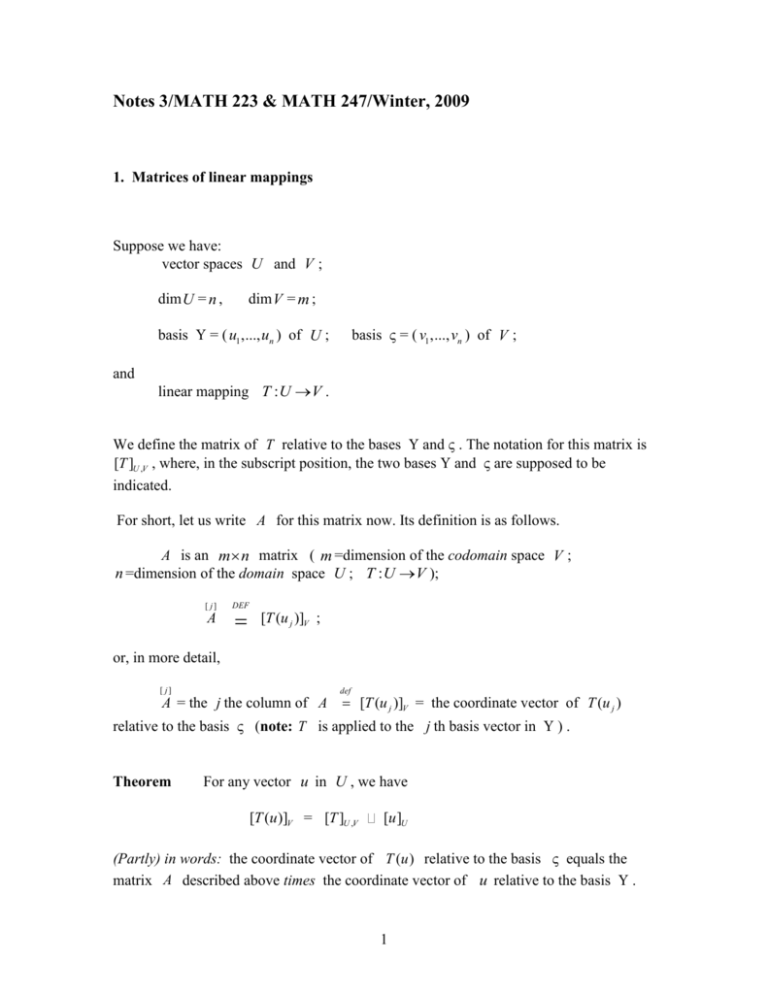
Notes 3/MATH 223 & MATH 247/Winter, 2009
1. Matrices of linear mappings
Suppose we have:
vector spaces U and V ;
dim U = n ,
dim V = m ;
basis = ( u1,..., un ) of U ;
and
basis = ( v1 ,..., vn ) of V ;
linear mapping T : U  V .
We define the matrix of T relative to the bases  and .The notation for this matrix is
[T ]U ,V , where, in the subscript position, the two bases and are supposed to be
indicated.
For short, let us write A for this matrix now. Its definition is as follows.
A is an m n matrix ( m =dimension of the codomain space V ;
n =dimension of the domain space U ; T : U  V );
[ j]
A
DEF

[T (u j )]V ;
or, in more detail,
[ j]
def
A = the j the column of A  [T (u j )]V = the coordinate vector of T (u j )
relative to the basis  (note: T is applied to the j th basis vector in ) .
Theorem
For any vector u in U , we have
[T (u )]V = [T ]U ,V
[u ]U
(Partly) in words: the coordinate vector of T (u ) relative to the basis equals the
matrix A described above times the coordinate vector of u relative to the basis  .
1
n
Let be ( x1,..., xn ) tr . Then u   x j  u j . Therefore, since T is linear,
Proof
j 1
T (u ) 
n
x
j 1
j
T (u j ) . Thus,
[T (u )]V 
n

j 1
x j  [T (u j )]V =
n
x
j 1
[ j]
j
 A = A  ( x1,..., xn ) tr = A  [u ]U .
Here, we made use of the fact that “taking coordinate vectors is a linear operation”:
[ w1  w2 ]V  [ w1 ]V  [ w21 ]V ;
and
[a  w]V  a  [ w]V .
Most common special case: when U  V , and  = . Now, T : V  V is a linear
operator. We abbreviate [T ]U ,V as [T ]U . The columns of [T ]U are the coordinate
vectors
[T (u j )]U , for j  1,..., n ; and the equality of the theorem becomes, for
arbitrary v in V :
[T (v)]U = [T ]U
[v]U .
Example 1. U = R 2 , V  R 3 ; n  2 , m  3 ; = (2) = (e1, e2 ) , the standard basis of R 2 ,
= (3) = (eˆ1 , eˆ2 , eˆ3 ) , the standard basis of R 3 ; T : R 2  R 3 defined by the formula
 x y 
 x


T ( )   x  2 y 
 y
 3x  4 y 


 1 0 
1
1


 
Now: T (e1 ) = T ( ) =  1  2  0  =  1  ;
0
 3 1  4  0 
 3 


 
2
 0 1 
1
0


T (e2 ) = T ( ) =  0  2 1  =  2 
1
 3  0  4 1
4


 
The matrix A = [T ]U ,V is
1 1
A = [ [T (e1 )]E , [T (e2 )]E ] = [ T (e1 ) , T (e2 ) ] =  1 2  .
 3 4 


 4
Given, as an example, u    , we have: [u ]U = [u ]E = u ;
7
 4  7   11 
 4 
 

T (u ) = T ( )   4  2  7  =  10  ; [T (u )]E = T (u ) =
 7   3  4  4  7  


  16 
 11 


 10  .
 16 


On the other hand:
1 1
A [u ]E = A u =  1 2 
 3 4 


 1 4  1 7 
 11 
 4




  =  1 4  2  7  =  10 
7
 (3)  4  4  7 
 16 




We see that the theorem is verified in this special case (which, of course, is not a proof of
the theorem itself). But we see even more: not only that the results of the two calculations
are the same, but also, that the intermediate expressions are also, essentially, the same.
The theorem itself has a very easy proof, one that is not more complicated than the
calculations above.
Example 2. The spaces U and V , as well as the mapping T the same as in Example
1; the bases   (u1, u2 ) ,   (v1, v2 , v3 ) consist of vectors defined as follows:
 2 
1
u1    , u2    ;
 1 
 3
1
 0
1
 
 
 
v1   0  , v2   2  , v3   1  .
 2 
1
 1
 
 
 
3
2  1


 3 
 2 


Now: T (u1 ) = T ( ) =   2  2  (1)  =  0  ;
 1 
 3  (2)  4  (1) 
2


 
 1 3 
4
1


 
T (u2 ) = T ( ) =  1  2  3  =  5 
 3
 3 1  4  3 
7


 
r
But, now we need [T (u1 )]V and [T (u2 )]V . If [T (u1 )]V =  s  , then
t 
 
 3 
1
 0
1






T (u1 ) =  0  = r  v1  s  v2  t  v3 = r   0   s   2   t   1  ;
2
 2 
1
 1
 
 
 
 
which means that (!)
 3 
1 0 1
  = 

0
0 2 1
2
 2 1 1
 


r
 
s
t 
 
1 0 1
Denoting the matrix  0 2 1  by P , and accepting the fact that P is invertible,
 2 1 1


this means that
r
  = 1
P
s
t 
 
 3 
 
0
2
 
[ P is the so-called transition, or change-of-basis, matrix for the change of basis from
, the standard basis in R 3 , to the “new” basis   (v1, v2 , v3 ) . Later, there will be more
on “change-of-basis”.]
We can calculate
4
P
1
 3 1 2 
=  2 1 1  ; and so
 4 1 2 


[T (u1 )]V
 r   3 1 2   3 
=  s  =  2 1 1   0  =
 t   4 1 2   2 
  
  
5
 .
4
 8 
 
Similarly,
[T (u2 )]V = P
1
 3 1 2   4 
 31 




T (u2 ) =  2 1 1   5  =  20  .
 4 1 2   7 
 35 

  


Thus, the matrix A = [T ]U ,V is
A =
[ [T (u1 )]V , [T (u2 )]V ] =
 5 31 


 4 20  .
 8 35 


The last matrix A can be used directly to calculate T (u ) if u is given in the form
u  a  u1  b  u2 ; the result will be given in the form T (u )  r  v1  s  v2  t  v3 .
3
For instance, let u  3  u1  5  u2 . Then [u ]U =   , and thus
 5 
 5 31 


[T (u )]V = A  [u ]U =  4 20 
 8 35 


 170 
3


  =  112  ,
 5 
 199 


which means that
T (u)  170  v1  112  v2  199  v3 .
If we want to check this result , then we calculate
 2 
1
 11 
u  3  u1  5  u2 = 3     5    = 
 ;
 1 
 3
 18 
5
(*)
from the definition of T directly:
11  18


 29 
 11 

 = 

T (u )  T (
25  ;
)   11  2  (18) 

 18 
 3  (11)  4  (18) 
 39 




On the other hand, from the formula (*)
1
0
1
 29 








T (u)  170  v1  112  v2  199  v3 = 170   0   112   2   199   1  =  25  ;
 2 
1
 1
 39 
 
 
 


unbelievably, the same!
U = R 23 , V = R 22 ;
Example 3.
= ( E1,1 , E1,2 , E1,3 , E2,1 , E2,2 , E2,3 ), the standard basis of R 23 :
1 0 0
0 1 0
0 0 1
E1,1  
 , E1,2  
 , E1,3  

0 0 0
0 0 0
0 0 0
0 0 0
 0 0 0
 0 0 0
E2,1  
 , E2,2  
 , E2,3  

1 0 0
0 1 0
0 0 1
= ( Eˆ1,1, Eˆ1,2 , Eˆ 2,1 , Eˆ 2,2 ), the standard basis of R 22 :
1 0 ˆ
0 1 ˆ
0 0 ˆ
0 0
Eˆ1,1  
 , E1,2  
 , E2,1  
 , E2,2  
 ;
0 0
0 0
1 0
0 1
T :R
23
R
22
1 2


defined by T ( X )  X  B , with the fixed matrix B   3 4  .
5 6


First of all, it is easy to see, without calculation, that T so defined is a linear mapping:
6
T ( X1  X 2 )  ( X1  X 2 )  B  X1  B  X 2  B  T ( X1 )  T ( X 2 ) ;
and similarly for the other condition.
We have that dim( U )=6 , dim( V )=4. thus, the matrix A  [T ]U ,V is a 4  6 matrix.
The columns of A are
[T ( E1,1 )]V , [T ( E1,2 )]V , [T ( E1,3 )]V , [T ( E2,1)]V , [T ( E2,2 )]V , [T ( E2,3 )]V .
We need to calculate the values at hand.
1 0 0
T ( E1,1 ) = 

0 0 0
1 2
1 2


ˆ
ˆ
ˆ
ˆ
=
3
4

 = 1 E1,1  2  E1,2  0  E2,1  0  E2,2 ,


0
0


5 6


0 1 0
T ( E1,2 ) = 

0 0 0
1 2
 3 4


ˆ
ˆ
ˆ
ˆ
=
3
4

 = 3  E1,1  4  E1,2  0  E2,1  0  E2,2 ,


0
0


5 6


0 0 1
T ( E1,3 ) = 

0 0 0
1 2
5 6


ˆ
ˆ
ˆ
ˆ
 3 4  =  0 0  = 5  E1,1  6  E1,2  0  E2,1  0  E2,2


5 6


0 0 0
T ( E2,1 ) = 

1 0 0
1 2

 0 0
ˆ
ˆ
ˆ
ˆ
 3 4  =  1 2  = 0  E1,1  0  E1,2  1 E2,1  2  E2,2

5 6 


0 0 0
T ( E2,2 ) = 

0 1 0
1 2

 0 0
ˆ
ˆ
ˆ
ˆ
3
4

 =  3 4  = 0  E1,1  0  E1,2  3  E2,1  4  E2,2

5 6 


0 0 0
T ( E2,3 ) = 

0 0 1
1 2

 0 0
ˆ
ˆ
ˆ
ˆ
 3 4  =  5 6  = 0  E1,1  0  E1,2  5  E2,1  6  E2,2 ;

5 6 


from which, the matrix A  [T ]U ,V is
7
1

2
A = 
0

0
3 5 0 0 0

4 6 0 0 0
0 0 1 3 5

0 0 2 4 6
2. Composition of linear mappings
Suppose we have vector spaces U , V , and W . Let us also suppose that we have
linear mappings S and T as in
S
T
U 
V 
W .
Then we can form the composite linear mapping
T S : U W ,
defined as follows:
(T S )(u )  T (S (u )) .
In other words, T S is applied to any u U by first applying S to u , and then,
applying T to the result S (u ) . Since the domain of T is supposed to coincide with
the codomain of S , the space V , and S (u ) is in V , T can be meaningfully applied
to S (u ) , and the result T ( S (u )) will be in W .
It is easy to see that S and T being linear implies that T S is a linear.
Let us now also assume that we have respective selected bases ,  and  of the
spaces U , V , and W . Then we can form the following matrices:
A  [S ]U ,V , B  [T ]V ,W , and
C  [T S ]
.
U ,W
(Note carefully the subscripts in these formulas. They are the only ones that are
meaningfully applicable in our context.)
8
Theorem
Under the above notation, C  B A . In an abbreviated notation:
[T S ]  [T ]
[S ]
Remark: the theorem says that “composition of linear mappings corresponds to matrix
multiplication.
Proof Let u be any vector in U . Let v  S (u ) . Then [v]V = [ S (u)]V  A[u]U . We
have [T (v)]W  B  [v]V . Therefore,
[(T S )(u)]W  [(T (S (u))]W  [(T (v)]W  B  [v]V =
!
= B  ( A [u ]U )  ( B  A)  [u ]U ;
at the exclamation mark, we used the associativity of matrix multiplication:
B  ( A  D)  ( B  A)  D ,
with D  [u ]U . We have shown that
[(T S )(u)]W = ( B  A)  [u ]U .
The definition of the matrix C says that
[(T S )(u)]W =
C  [u]U .
Therefore ( B  A)  [u ]U = C  [u]U . Since this holds true for all u in U , we must have
that C  B A , as asserted.
9