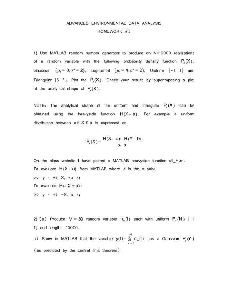
ADVANCED ENVIRONMENTAL DATA ANALYSIS
HOMEWORK #2
1) Use MATLAB random number generator to produce an N=10000 realizations
of a random variable with the following probability density function
Gaussian
(1 = 0;  2 = 2) ,
Lognormal
(1 =
4;  2 = 2),
Px (X ) :
Uniform [-1 1] and
Triangular [5 7]. Plot the Px (X ) . Check your results by superimposing a plot
of the analytical shape of Px (X ) .
NOTE: The analytical shape of the uniform and triangular
obtained
using
the
heavyside
function
H (X - a) .
For
Px (X )
example
a
can be
uniform
distribution between a £ X £ b is expressed as:
Px (X ) =
H (X - a ) - H (X - b)
b- a
On the class website I have posted a MATLAB heavyside function utl_H.m.
To evaluate H (X - a) from MATLAB where X is the x-axis:
>> y = H( X, -a );
To evaluate H (- X + a) :
>> y = H( -X, a );
2) (a) Produce M = 30 random variable nm (t ) each with uniform Pn (N ) [-1
1] and length
10000.
a) Show in MATLAB that the variable y(t ) =
M
å
m= 1
(as predicted by the central limit theorem).
nm (t ) has a Gaussian Py (Y )
b) Now assume Pn (N ) is Gaussian
Pz (Z ) of the variable
z(t ) =
M
å
(1 = 0;  2 = 1) .
nm2 (t ) . Verify that
Compute in MATLAB
Pz (Z ) is a chi-square
m= 1
distribution by superimposing a plot of the analytical shape.
3) Now assume that you have measured a random variable x(t ) along with its
statistics. You find that Px (X ) is a uniform distribution between [-1 1] and
that each value of x(ti ) is independent of each other (in other words x(t )
has no autocorrelation in time). What are the statistics of the variable y(t )
given by the following equation:
y(t ) =
dx
dt
HINT: Remember that you can discretize the equation y(t i ) =
x(t i + 1 ) - x(t i )
and
dt
that x(ti + 1 ) and x(ti ) can be considered independent random variables with
known Px (X ) = Pxi (X i ) = Pxi + 1 (X i + 1 ). If you have trouble with the math, find the
Py (Y ) numerically using MATLAB. Once you know the shape of it try to see if
you can derive the same result analytically.
4) In class we have quantified the linear relationship between two variables x '
and
y'
with
x' = y' = 0,
using
the
correlation
coefficient.
If
a
linear
relationship exists, than one could write a statistical optimal linear estimator by
imposing the following model (see chap. 3 Davis on class website):
yˆ ¢=  x ¢
where  =
x ¢y ¢
x ¢2
This fundamental result can be obtained using the least square approach and
minimizing
M
J=
å
i=1
the
M
ni2 =
å (y ¢i
expected
2
 xi¢)
value
J
of
the
cost
function
with respect to  , where n = y¢- yˆ¢= y¢- x¢ is the
i=1
residual between the model estimate ŷ ¢ and the observed value y ¢. Show
analytically
or
numerically
that
when
the
model
errors
ni
are
normally
distributed, the estimate ŷ ¢= x ¢ is equivalent to the estimate obtained using
the conditional probability density function
yˆ ¢=  x ¢=
ò
+¥
- ¥
Y ¢ Py|x (Y ¢|X ¢= x ¢)dY ¢
Now show that this is no longer true when the errors are lognormally
distributed.
5) Download the MATLAB function hw2_generate_Y.m and bs_rand.m. This
function will generate 4 different sets of observations of a variable y along with
the standard deviation of the measurement error n .
a) Using the least square approach and chi-square statistics, test which of the
two models y(t ) = a + bt + n(t ) and y(t ) = a + bt + ct 2 + n (t )
is consistent with
each of the observational data sets. Compute the uncertainty of the model
parameters.
In MATLAB to generate a realization for set number one
>> set_number = 1;
>> [y,t,n_std] = hw2_generate_Y(set_number);
You can generate many realizations of data set number one by just calling this
function over and over again. You will need to do this to test the chi-square
statistics of the cost function J =
M
å
n (t i )2 .
i=1
You will do the same test for observational set number 2, 3 and 4.
>> set_number = 2;
>> [y,t,n_std] = hw2_generate_Y(set_number);
b) Explain why the expected value of J is inferred by chi-square statistics.
J =
ò
+¥
- ¥
J PJ (J )dJ
where PJ (J ) = chi - square(r )
and r is the degrees of freedom.
OPTIONAL STUDY PROBLEMS- NOT REQUIRED
1) Prove that the moments of a random variable x with a Gaussian Px (X ) can
be determined only by the mean m1 and the variance  2 . Compute also the
value of m3 .
Px (X ) =
2) Random variable
X
has
é (X - m )2 ù
1
1 ú
exp êê2
údX
2
2
êë
ú
û
Px (X ) =  (X 2 -  2 ) . Compute the probability
density function of the two new random variables Y and Z defined as:
Y =
1
(X 1 + X 2 )
3
Z=
X 1X 2
2
where X n are assumed to be independent realizations of the random variable X.