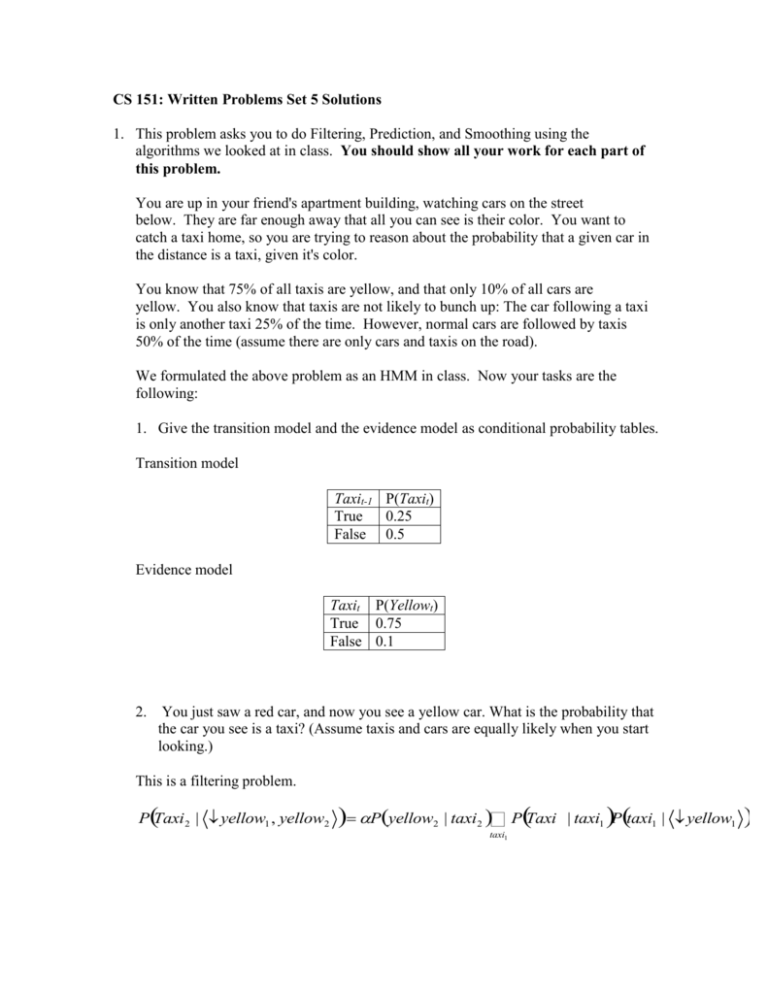
CS 151: Written Problems Set 5 Solutions
1. This problem asks you to do Filtering, Prediction, and Smoothing using the
algorithms we looked at in class. You should show all your work for each part of
this problem.
You are up in your friend's apartment building, watching cars on the street
below. They are far enough away that all you can see is their color. You want to
catch a taxi home, so you are trying to reason about the probability that a given car in
the distance is a taxi, given it's color.
You know that 75% of all taxis are yellow, and that only 10% of all cars are
yellow. You also know that taxis are not likely to bunch up: The car following a taxi
is only another taxi 25% of the time. However, normal cars are followed by taxis
50% of the time (assume there are only cars and taxis on the road).
We formulated the above problem as an HMM in class. Now your tasks are the
following:
1. Give the transition model and the evidence model as conditional probability tables.
Transition model
Taxit-1 P(Taxit)
True
0.25
False 0.5
Evidence model
Taxit P(Yellowt)
True 0.75
False 0.1
2.
You just saw a red car, and now you see a yellow car. What is the probability that
the car you see is a taxi? (Assume taxis and cars are equally likely when you start
looking.)
This is a filtering problem.
P(Taxi 2 | Øyellow1 , yellow2
)= aP(yellow
2
| taxi2 )å P(Taxi | taxi1 )P(taxi1 | Øyellow1
taxi1
)
PTaxi1 | yellow1   P yellow1 | taxi1  PTaxi1 | taxi0 Ptaxi0 
taxi0
  .25,.9  .25,.75  .5  .5,.5  .5   .09375,.5625  .143,.857
PTaxi 2 | yellow1 , yellow2
   .75,.1  .25,.75  .143 
.5,.5  .857   .3482,.0536  .867,.133
3. What is the probability that the next car will be a taxi?
This is a prediction problem.
PTaxi3 | yellow1 , yellow 2     PTaxi3 | taxi2 Ptaxi2 | yellow1 , yellow 2

taxi2
   .25,.75  .867  .5,.5  .133  .283,.717
4. You decide not to go down, and you observe that the next (third) car is also
yellow. Use this new information to update your belief that the last car (the
second car) you saw was a taxi.
This is a smoothing problem. We can take the forward messages from the probability
we calculated in part 2 (or we can just use the final distribution since we will renormalize). We just need to calculate the backwards message.
P yellow 3 | Taxi2    P yellow 3 | taxi3  1  Ptaxi3 | Taxi2 
taxi3
 .75  .25,.5  .1  .75,.5  .2625,.425
PTaxi2 | yellow1 , yellow2 , yellow3    .867,.133  .2625,.425  .801,.199
5. Explain quatlitatively why your new estimate in problem 4 makes sense, given
your evidence and transition models (I am looking for an English description
here).
Our probability that car 2 was a taxi has decreased after receiving the information that
car 3 was yellow. This makes sense because taxis are unlikely to bunch up, so seeing
two of them in a row doesn’t make sense. So after seeing the second red car you
become less sure that you saw a taxi, in effect because your data doesn’t fit the model
very well—your evidence model is essentially competing with your transition model,
and they are kind of cancelling each other out a bit.
2. from http://www-nlp.stanford.edu/~grenager/cs121//handouts/hw3_solutions.pdf
An appealing use of HMMs is for localization: in other words, given a map, and a set of
observations of your environment, figure out where you are. Suppose we are walking
around the Claremont Colleges campus, which is roughly a 1x1 mile square (5280 feet by
5280 feet) (OK, not quite, but close enough...). We’ve been given a map, and we’d like to
figure out where we are every ten seconds, down to a resolution of 1 foot.
(a) Let’s formalize this as an HMM. What does each of the hidden states Xt represent?
What is the domain of each state variable? How big is this domain?
Each state Xt represents the location at time t. The domain is a position in the grid,
the set of 1x1 foot squares on the campuses. The size of the domain is 52802.
(b) Suppose that we’re walking with a blindfold on, at roughly 2 miles per hour,
trying to go straight. You can ignore obstacles (such as buildings) for now. What’s a
reasonable transition model, P(Xt|Xt−1)?
Since we don’t know what direction we’re walking in, the transition model should
give equal probability to all of the squares roughly 15 feet away, since 2 miles an
hour is about 1.5 feet per second.
(c) Assume that we get dropped off somewhere on the campus blindfolded but we
don’t know where. What’s a good starting distribution P(X1)?
A uniform distribution.
(d) Suppose that every ten seconds we can stop and take our blindfold off, and look
for Smith
Tower (on Pomona's campus). If we can see it, we measure approximately how far
away it is by measuring its apparent height. We then report the approximate distance
in 100 foot increments. What should each evidence variable Et represent? What is the
domain of each evidence variable? How big is this domain?
Each Et should be the distance from Smith tower. The domain is [0, 100, 200, …,
7500] (the length of the diagonal of the space—we’d never be this far away, but we
certainly can’t be farther). The size of the domain is 75.
(e) Formalize the emission model P(Et|Xt).
Again, since we don’t know which direction we are from the tower, we would have a
ring of equal probability at all the positions that are Et away from the tower, with
some smoothing for measurement error. If we assume we can tell the direction (e.g.,
we have a compass or something) then Et gives us Xt, with some smoothing around
that position to account for noise.
(f) Suppose we walk “straight” for 1 minute (60 seconds). How many computations
will the forward algorithm take to compute a distribution over our possible locations
at the last time step?
(Hint: this is the “filtering” task from lecture.) Given a computer that can process 1
billion computations per second, how long will this computation take?
We know that each step of filtering takes time O(k2). So here k= 28 M= 225, and thus
filtering will take on the order of 250 computations. Since we can do approximately 1
billion, or 230, operations per second, a single step of filtering for this task should take
220 or 1 million seconds, which is approximately 120 days. But we want to do
60/10= 6 filtering steps, which should take us approximately two years. So, we can’t
really run this exact algorithm in real time to localize ourselves.