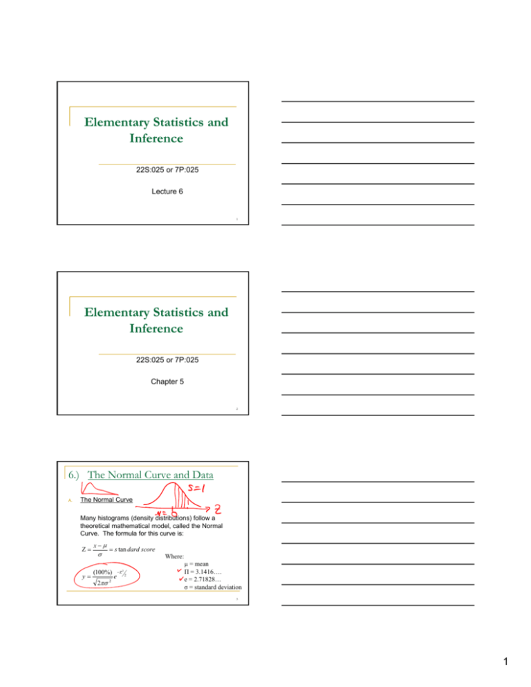
Elementary Statistics and
Inference
22S:025 or 7P:025
Lecture 6
1
Elementary Statistics and
Inference
22S:025 or 7P:025
Chapter 5
2
6.) The Normal Curve and Data
A.
The Normal Curve
Many histograms (density distributions) follow a
theoretical mathematical model, called the Normal
Curve The formula for this curve is:
Curve.
Ζ=
y=
x−μ
σ
= s tan dard score
(100%)
2πσ 2
e
−Ζ
2
2
Where:
µ = mean
Π = 3.1416….
e = 2.71828…
σ = standard deviation
3
1
6.) The Normal Curve and Data (cont.)
We can use this model be referring to a table on page
A104 that provides the percentage of scores between
the mean and plus or minus a given number of standard
score units from the mean.
4
6.) The Normal Curve and Data (cont.)
Partial Table (from A104)
Z
1 00
1.00
Height of
Curve
24 20
24.20
Area Between
±Z
68 27%
68.27%
1.65
10.23
90.11%
1.95
5.96
94.88%
2.00
5.40
95.45%
2.60
1.36
99.07%
5
6.) The Normal Curve and Data (cont.)
„
The normal curve is symmetric and bell-shaped, with the
mean as the point of symmetry. (See the diagram in
Figure 1 – page 79)
„
The p
percentage
g of scores between the mean and one
standard score unit above the mean is about 34.
„
Within one standard deviation of the mean, about 68% of
the scores occur when the density distribution
(histogram) is normal.
6
2
6.) The Normal Curve and Data (cont.)
7
6.) The Normal Curve and Data (cont.)
Note: When the scores in a histogram are converted to
standard scores, the mean of the standard scores is
“Ø”, and the standard deviation is “1”. In a distribution
of standard scores, 68% are within one standard
deviation of the mean, and 95% are within 2 standard
deviations of the mean.
mean See the diagram of Figure 1
1,
page 79.
ƒ For a woman who was 69.5 inches tall, she was 2
standard deviations above the mean, and about 97.5%
of the women were shorter than her. About 2 ½ % of
the women were taller than 69.5 inches. (See diagram
on page 81 – Figure 2)
8
6.) The Normal Curve and Data (cont.)
B.
Finding Areas Under the Normal Curve
ƒ
Find percent of scores between mean and 1 SD above
the mean.
34%
0
1
9
3
6.) The Normal Curve and Data (cont.)
„
Find the percent of scores greater than 1 standard
deviation above the mean – about 16%.
„
The percent of scores within 1 SD of the mean – 68%.
„
The percent of scores less than 1 SD below the mean –
about 16%.
Note: See other examples on pages 82-84.
Exercise Set B – (pages 84-85) #1, 2, 3, 4, 5
10
6.) The Normal Curve and Data (cont.)
C.
Normal Approximation for Data
„
HANES data – For men age 18-74,
Average height = 69 inches
SD = 3 inches
And the heights were approximately normal in shape.
11
6.) The Normal Curve and Data (cont.)
„
The approximate percentage of men with heights
between 63 and 72 inches can be found by using the
normal curve table for percentage between ± 1 standard
score from the mean.
x−μ
63 − 69 − 6
=
= −2.00
3
3
x − μ 72 − 69 3
Ζ=
=
= = 1.00
3
3
σ
Ζ=
σ
=
12
4
6.) The Normal Curve and Data (cont.)
95%
47.5%
-2.00
2.00
0
68%
34%
-1.00
0
1.00
Total =47.5 + 34 = 81.5 or 82%
13
6.) The Normal Curve and Data (cont.)
„
This use [ distribution) approximates the normal
distribution in slope.
If the histogram is skewed, the normal approximation will
not work.
work
Exercise Set C – (page 88) #1, 2, 3
14
5