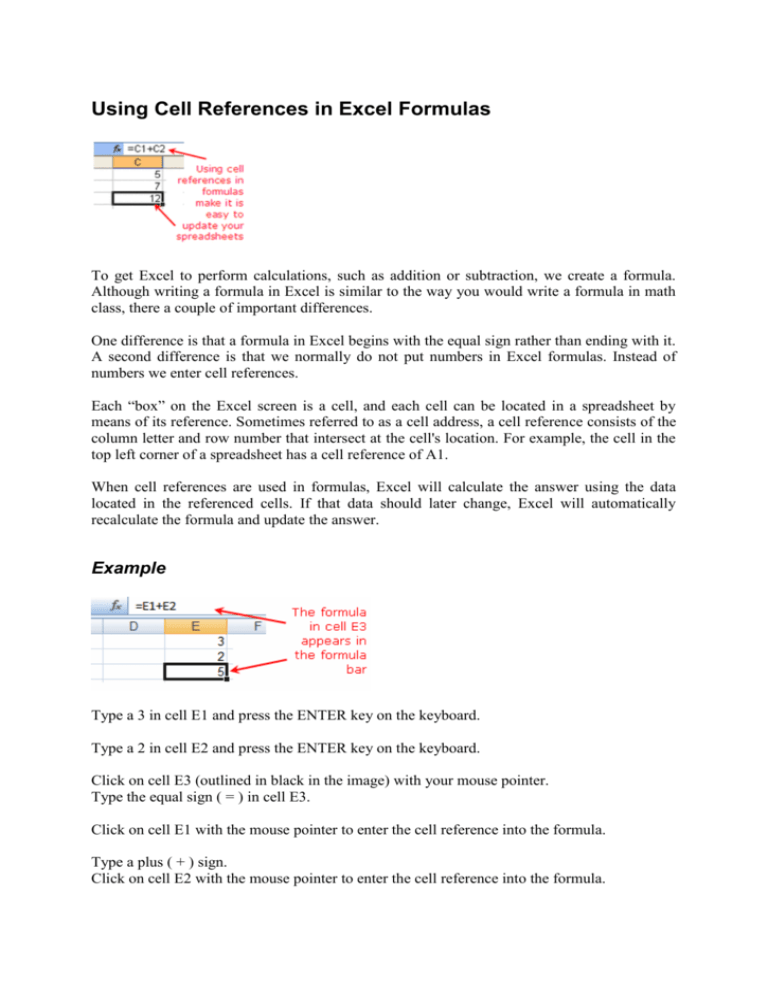
Using Cell References in Excel Formulas
To get Excel to perform calculations, such as addition or subtraction, we create a formula.
Although writing a formula in Excel is similar to the way you would write a formula in math
class, there a couple of important differences.
One difference is that a formula in Excel begins with the equal sign rather than ending with it.
A second difference is that we normally do not put numbers in Excel formulas. Instead of
numbers we enter cell references.
Each “box” on the Excel screen is a cell, and each cell can be located in a spreadsheet by
means of its reference. Sometimes referred to as a cell address, a cell reference consists of the
column letter and row number that intersect at the cell's location. For example, the cell in the
top left corner of a spreadsheet has a cell reference of A1.
When cell references are used in formulas, Excel will calculate the answer using the data
located in the referenced cells. If that data should later change, Excel will automatically
recalculate the formula and update the answer.
Example
Type a 3 in cell E1 and press the ENTER key on the keyboard.
Type a 2 in cell E2 and press the ENTER key on the keyboard.
Click on cell E3 (outlined in black in the image) with your mouse pointer.
Type the equal sign ( = ) in cell E3.
Click on cell E1 with the mouse pointer to enter the cell reference into the formula.
Type a plus ( + ) sign.
Click on cell E2 with the mouse pointer to enter the cell reference into the formula.
Press the ENTER key on the keyboard.
The answer 5 should appear in cell E3.
Click on cell E3. The formula = E1 + E2 is shown in the formula bar above the worksheet.
Exercise 1
On the first worksheet perform the following calculation
Relative and absolute references
By default, a spreadsheet cell reference is relative. What this means is that as a formula or
function is copied and pasted to other cells, the cell references in the formula or function
change to reflect the function's new location.
In contrast, an absolute cell reference does not change when it a formula is copied and pasted
to other cells.
A relative cell reference consists of the column letter and row number that intersect at the
cell's location.
An example of a relative cell reference would be C4, G15, or Z2345.
absolute cell reference identifies the location a cell or group of cells.
Cell references are used in formulas, functions, charts, and other Excel commands.
An absolute cell reference consists of the column letter and row number surrounded by dollar
signs ( $ ).
An example of an absolute cell reference would be $C$4, $G$15, or $A$345.
Note: An easy way to add the dollar signs to a cell reference is to click on a cell reference and
then press the F4 key on the keyboard.
An absolute cell reference is used when you want a cell reference to stay fixed on a specific
cell.
This means that as a formula or function is copied and pasted to other cells, the cell references
in the formula or function do not change.
By contrast, most cell references in a spreadsheet are relative cell references, which change
when copied and pasted to other cells.
Exercise 2
On the second worksheet, create the following table:
Enter the appropriate formula to calculate the vat, and then with fill handle, copy it to the next
cell.
Enter the appropriate formula to calculate the gross price, and then with fill handle, copy it to
the next cell.
SUM, MAX, MIN and AVERAGE Functions
Excel SUM Function
Calculations in Excel are often used to total a column or a row of data. The Excel SUM
function offers a shortcut to adding up these columns and rows of data.
If we were to create a formula that adds up the contents of cells B7 to B10, the formula would
be:
=B7+B8+B9+B10
Writing this takes some time even if we are using pointing to add cell references. Also, the
longer the formula, the greater the potential for errors being introduced.
The SUM function allows us to write only the start and end points of the data range separated
by a colon ( : ) and the function will add together the contents of all the cells in the range.
The same formula, written using the SUM function would be:
= SUM(B7 : B10)
Excel MAX Function
The MAX function, one of Excel's statistical functions, is used to find the largest or maximum
number in a given list of values or arguments.
The syntax for the MAX function is:
=MAX( argument1, argument2, ... argument30 )
Argument1, argument2, ... argument30 can be numbers, named ranges, arrays, or cell
references. Up to 30 arguments can be entered.
Example Using Excel's MAX Function:
1.Enter the following data into cells C1 to C6: 114,165,178,143,130,167.
2.Click on cell C7 - the location where the results will be displayed.
3.Type = max( in cell C7.
4.Drag select cells C1 to C6 with the mouse pointer.
5.Type the closing bracket " ) " after the cell range in cell C7.
6.Press the ENTER key on the keyboard.
7.The answer 178 appears in cell C7.
8.The complete function = MAX ( C1 : C6 ) appears in the formula bar.
You can also insert MAX function another way:
1.Enter the following data into cells C1 to C6: 114,165,178,143,130,167.
2.Click on cell C7 - the location where the results will be displayed.
3.Choose Insert/Function
4.Choose Category > Statistical.
5.Click on MAX in the list to bring up the function's dialog box.
6.Drag select cells C1 to C6 on the spreadsheet to enter the range into the dialog box.
7.Click OK.
8.The answer 178 should appear in cell C7 as it is the largest number in the selected range.
9.When you click on cell C7 the complete function = MAX (C1 : C6) appears in the formula
bar above the worksheet.
Excel MIN Function
The MIN function, one of Excel’s statistical functions, is used to find the smallest or
minimum value in a given list of numbers or arguments.
The syntax for the MIN function is:
=MIN ( argument1, argument2, ... argument30 )
Argument1, argument2, ... argument30 can be numbers, named ranges, arrays, or cell
references. Up to 30 arguments can be entered.
Example Using Excel's MIN Function:
1.Enter the following data into cells C1 to C6: 114,165,178,143,130,167.
2.Click on cell C7 - the location where the results will be displayed.
3.Type “=min(” in cell C7.
4.Drag select cells C1 to C6 with the mouse pointer.
5.Type the closing bracket " ) " after the cell range in cell C7.
6.Press the ENTER key on the keyboard.
7.The answer 114 appears in cell C7.
8.The complete function =MIN(C1:C6) appears in the formula bar.
You can also insert MIN function choosing Insert/Function the same way like in MAX
function example.
Excel AVERAGE Function
The AVERAGE function can be used to find the average, or arithmetic mean, of values in a
selected range of cells.
The function is written as follows:
= AVERAGE (argument)
The argument for this function is data contained in the selected range of cells.
Example Using Excel's AVERAGE Function:
1.Enter the following data into cells C1 to C6: 11,12,13,14,15,16.
2.Click on cell C7 - the location where the results will be displayed.
3.Type " = average( " in cell C7.
4.Drag select cells C1 to C6 with the mouse pointer.
5.Type the closing bracket " ) " after the cell range in cell C7.
6.Press the ENTER key on the keyboard.
7.The answer - 13.5 - should be displayed in cell C7.
8.The complete function = AVERAGE (C1 : C6) appears in the formula bar above the
worksheet.
You can also insert AVERAGE function choosing Insert/Function the same way like in MAX
function example.
Exercise 3
In the previous exercise calculate sum, minimum, maximum and average.
Excel IF Function
The IF function, one of Excel's logical functions, tests to see if a certain condition in a
spreadsheet is true or false.
The syntax for the IF function is:
=IF ( logical_test; value_if_true; value_if_false )
logical_test - a value or expression that is tested to see if it is true or false.
value_if_true - the value that is displayed if logical_test is true.
value_if_false - the value that is displayed if logical_test is false.
Example Using Excel's IF Function:
1.Enter 35 into cell D1.
2.Click on cell E1 - the location where the results will be displayed.
3.Choose Insert/Function
4.Choose Category Logical.
5.Click on IF in the list to bring up the function's dialog box.
6.On the Logical_test line in the dialog box, click on cell D1. After this type the less than
symbol ( < ) and then the number 26.
7.On the Value_if_true line of the dialog box, type 100.
8.On the Value_if_false line of the dialog box, type 200.
9.Click OK.
10.The value 200 should appear in cell E1, since the value in D1 is greater than 26.
Changing the IF Function's Results
1.To change the result in cell E1, change the number in cell D1. For example, change E1 to 15
and press the Enter key.
2.The value 100 should now be present in cell E1 since the value in D1 is now less than 26.
3.If you click on cell E1, the complete function = IF ( D1 < 26 ; 100 ; 200 ) appears in the
formula bar above the worksheet.
Performing calculations
The IF function can perform different calculations depending on whether the function returns
a true value or not.
The example below uses different deduction rates in its calculations based on employee
income.
=IF(A5 < 29701; A5 * 15%; A5 * 25%)
If employees earn above a certain level, one deduction rate will be used in the calculation, if
their income is below this level, a different deduction rate will be used.
What the above example does is test to see if the value in cell A5 is less than 29,701. If it is,
the function multiplies the value in cell A5 by 15%(the "value if true" argument). If the value
in A5 is greater than or equal to 29,701, then the amount in cell A5 is multiplied by 25% (the
"value if false" argument).
Displaying text
Having text displayed by an IF function rather than a number can make it easier to find and
read specific results in the spreadsheet.
Below, the example IF function is setup to test whether a student's mark is greater than or
equal to 50. If it is, "Passed" is written into the target cell. If not, the word "Failed" appears.
=IF(A5>=50;”Passed”;”Failed”)
A second example could be used by a company to quickly determine which employees are
entitled to a bonus for exceeding a certain level of production.
=IF(A5>=5000;”Pay Bonus”;”No Bonus”)
Note: when you want to use text in an IF function each text statement must be enclosed in
quotes, such as "Pay Bonus".
Exercise 4
Using IF function, calculate if gross price of each item is higher or lower then average.
Exercise 5
Create the following table and then calculate the average ratings for each student, and for each
subject. In the column scholarship, type YES or NO depending on whether the student's
average score is greater than 4.0.