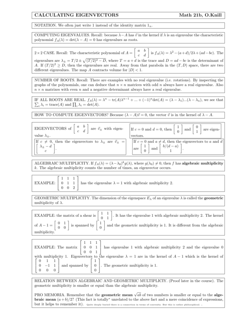
CALCULATING EIGENVECTORS
Math 21b, O.Knill
NOTATION. We often just write 1 instead of the identity matrix 1 n .
COMPUTING EIGENVALUES. Recall: because λ−A has ~v in the kernel if λ is an eigenvalue the characteristic
polynomial fA (λ) = det(λ − A) = 0 has eigenvalues as roots.
a b
2 × 2 CASE. Recall: The characteristic polynomial of A =
is fA (λ) = λ2 − (a + d)/2λ + (ad − bc). The
c d
p
eigenvalues are λ± = T /2 ± (T /2)2 − D, where T = a + d is the trace and D = ad − bc is the determinant of
A. If (T /2)2 ≥ D, then the eigenvalues are real. Away from that parabola in the (T, D) space, there are two
different eigenvalues. The map A contracts volume for |D| < 1.
NUMBER OF ROOTS. Recall: There are examples with no real eigenvalue (i.e. rotations). By inspecting the
graphs of the polynomials, one can deduce that n × n matrices with odd n always have a real eigenvalue. Also
n × n matrixes with even n and a negative determinant always have a real eigenvalue.
IF
REAL. fA (λ) = λn − tr(A)λn−1 + ... + (−1)n det(A) = (λ − λ1 )...(λ − λn ), we see that
P ALL ROOTS AREQ
i λi = trace(A) and
i λi = det(A).
HOW TO COMPUTE EIGENVECTORS? Because (λ − A)~v = 0, the vector ~v is in the kernel of λ − A.
EIGENVECTORS of
value λ± .
a
c
b
d
are ~v± with eigen-
If c = 0 and d = 0, then
vectors.
If
c 6= 0, then the eigenvectors to λ± are ~v± =
λ± − d
.
c
1
0
and
0
1
are eigen-
If c = 0 and
a 6=
d, then the eigenvectors to a and d
b/(d − a)
1
.
and
are
1
0
ALGEBRAIC MULTIPLICITY. If fA (λ) = (λ−λ0 )k g(λ), where g(λ0 ) 6= 0, then f has algebraic multiplicity
k. The algebraic multiplicity counts the number of times, an eigenvector occurs.


1 1 1
EXAMPLE:  0 1 1  has the eigenvalue λ = 1 with algebraic multiplicity 2.
0 0 2
GEOMETRIC MULTIPLICITY. The dimension of the eigenspace E λ of an eigenvalue λ is called the geometric
multiplicity of λ.
1 1
. It has the eigenvalue 1 with algebraic multiplicity 2. The kernel
EXAMPLE: the matrix of a shear is
0 1
1
0 1
and the geometric multiplicity is 1. It is different from the algebraic
is spanned by
of A − 1 =
0
0 0
multiplicity.

1 1
EXAMPLE: The matrix  0 0
0 0
with
multiplicity
1.
Eigenvectors



0 1 1
 0 −1 1  and spanned by 
0 0 0

1
1  has eigenvalue 1 with algebraic multiplicity 2 and the eigenvalue 0
1
to the eigenvalue λ = 1 are in the kernel of A − 1 which is the kernel of
1
0 . The geometric multiplicity is 1.
0
RELATION BETWEEN ALGEBRAIC AND GEOMETRIC MULTIPLICIY. (Proof later in the course). The
geometric multiplicity is smaller or equal than the algebraic multiplicity.
√
PRO MEMORIA. Remember that the geometric mean ab of two numbers is smaller or equal to the algebraic mean (a + b)/2? (This fact is totally∗ unrelated to the above fact and a mere coincidence of expressions,
but it helps to remember it). Quite deeply buried there is a connection in terms of convexity. But this is rather philosophical. .



EXAMPLE. What are the algebraic and geometric multiplicities of A = 


2
0
0
0
0
1
2
0
0
0
0
1
2
0
0
0
0
1
2
0
0
0
0
1
2



?


SOLUTION. The algebraic multiplicity of the eigenvalue 2 is 5. To get the kernel of A − 2, one solves the system
of equations x4 = x3 = x2 = x1 = 0 so that the geometric multiplicity of the eigenvalues 2 is 4.
CASE: ALL EIGENVALUES ARE DIFFERENT.
If all eigenvalues are different, then all eigenvectors are linearly independent and all geometric and algebraic multiplicities are 1.
PROOF.
from 0 and
Pare linearly dependent. We have
P assume the eigenvectors
P
P Let λi be an eigenvalue different
vi = j6=i bj vj with bP
vi = j6=i aj vj and λi vi = Avi = A( j6=i aj vj ) = j6=i aj λj vj so that P
j = aj λj /λi .
a
v
from
v
=
If the
eigenvalues
are
different,
then
a
=
6
b
and
by
subtracting
v
=
j
j
i
j
j
i
j6=i bj vj , we get
j6=i
P
0 = j6=i (bj − aj )vj = 0. Now (n − 1) eigenvectors of the n eigenvectors are linearly dependent. Use induction.
CONSEQUENCE. If all eigenvalues of a n × n matrix A are different, there is an eigenbasis, a basis consisting
of eigenvectors.
EXAMPLE. A =
1
0
1
3
has eigenvalues 1, 3 to the eigenvectors
1
0
−1
1
.
EXAMPLE. (See homework problem 40 in the book).
Photos
of
the
Swiss lakes in the
text. The pollution
story is fiction
fortunately.
The vector
An (x)b gives
levels

 the pollution

 in the three lakes (Silvaplana, Sils, St Moritz) after n weeks, where
0.7 0
0
100
A =  0.1 0.6 0  and b =  0  is the initial pollution.
0 0.2 0.8
0
100
80
60
40
20


0
There is an eigenvector e3 = v3 =  0  to the eigenvalue λ3 = 0.8.
1




0
1
There is an eigenvector v2 =  1  to the eigenvalue λ2 = 0.6. There is further an eigenvector v1 =  1 
−1
−2
to the eigenvalue λ1 = 0.7. We know An v1 , An v2 and An v3 explicitly.
How do we get the explicit solution An b? Because b = 100 · e1 = 100(v1 − v2 + 3v3 ), we have
4
6
An (b) =
8
10
100An (v1 − v2 + 3v3 ) = 100(λn1 v1 − λn2 v2 + 3λn3 v3 )






 

1
0
0
100(0.7)n

100(0.7n + 0.6n )
= 100 0.7n  1  + 0.6n  1  + 3 · 0.8n  0  = 
n
n
n
−2
−1
1
100(−2 · 0.7 − 0.6 + 3 · 0.8 )