Statistics 200 Homework 5 Solutions
Nicolas Annoni
March 6, 2008
1
Problem 9.6
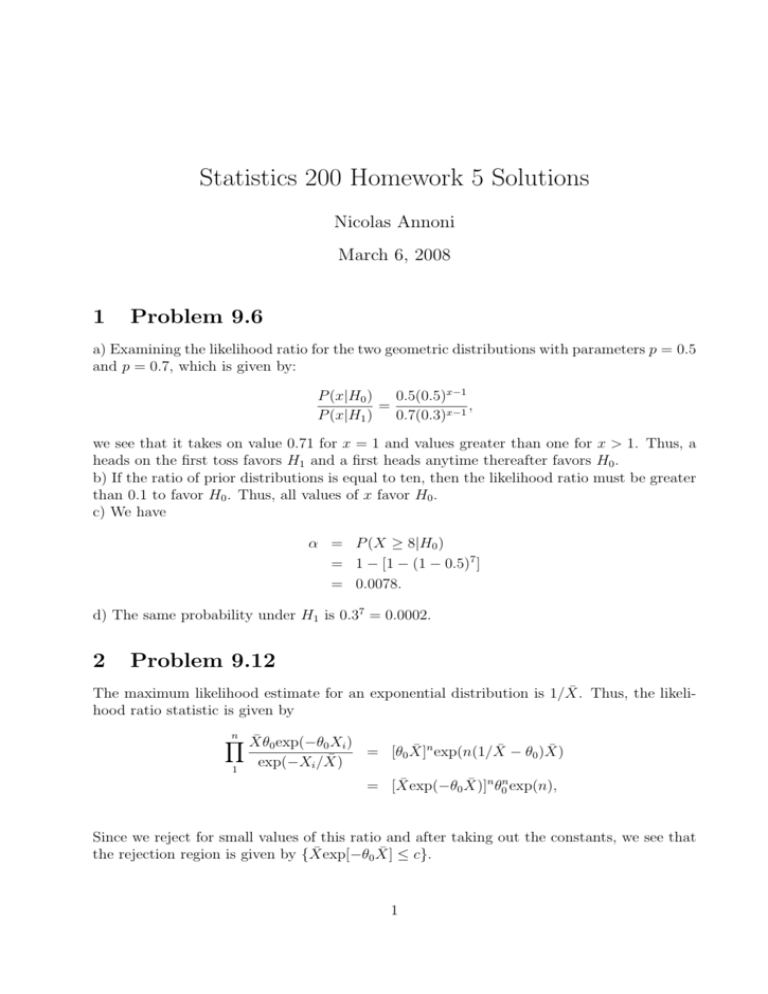
a) Examining the likelihood ratio for the two geometric distributions with parameters p = 0.5
and p = 0.7, which is given by:
P (x|H0 )
0.5(0.5)x−1
=
,
P (x|H1 )
0.7(0.3)x−1
we see that it takes on value 0.71 for x = 1 and values greater than one for x > 1. Thus, a
heads on the first toss favors H1 and a first heads anytime thereafter favors H0 .
b) If the ratio of prior distributions is equal to ten, then the likelihood ratio must be greater
than 0.1 to favor H0 . Thus, all values of x favor H0 .
c) We have
α = P (X ≥ 8|H0 )
= 1 − [1 − (1 − 0.5)7 ]
= 0.0078.
d) The same probability under H1 is 0.37 = 0.0002.
2
Problem 9.12
The maximum likelihood estimate for an exponential distribution is 1/X̄. Thus, the likelihood ratio statistic is given by
n
Y
X̄θ0 exp(−θ0 Xi )
1
exp(−Xi /X̄)
= [θ0 X̄]n exp(n(1/X̄ − θ0 )X̄)
= [X̄exp(−θ0 X̄)]n θ0n exp(n),
Since we reject for small values of this ratio and after taking out the constants, we see that
the rejection region is given by {X̄exp[−θ0 X̄] ≤ c}.
1
3
Problem 9.18
The likelihood ratio statistic is given by
n
Y
λ0 exp(−λ0 |Xi |)
1
λ1 exp(−λ1 |Xi |)
=[
X
λ0 n
] exp[(λ1 − λ0 )
|Xi |]
λ1
P
Because
λ
>
λ
,
this
test
rejects
only
when
|Xi | < c with c determined by the equation
1
0
P
P ( |Xi | < c|H0 ) = α. Because we set c using the null hypothesis and because the test is
the same for all λ1 > λ0 , the test is uniformly most powerful.
4
9.20
By the Neyman–Pearson Lemma, the likelihood ratio test has power greater than or equal to
the power of any other test for two simple hypotheses. Thus, we must merely calculate this
test’s power. We see that the condition 1/2X ≤ C0 is equivalent to the condition X > C for
a different constant C. To find this constant, set P (X > C|H0 ) = 0.10. Because f0 specifies
the uniform distribution, the constant must be 0.9. Then, the power is
Z 1
P (X > 0.9|H1 ) =
2xdx
0.9
= 0.19.
5
9.32
a) After dividing normal density A by normal density B and using X = 120, we receive a
likelihood ratio of exp(−3/10).
b) This is an application of Bayes’ Rule. We have:
f (X|B)P (B)
f (X|B)P (B) + f (X|A)P (A)
−25
exp( 2·25
2)
=
−25
−400
exp( 2·252 ) + exp( 2·25
2)
= 0.574
P (B|X) =
The question does not specify the null hypothesis, so there could be two sets of answers,
depending upon whether one chooses A or B to be in the null hypothesis. If A is in the null
hypothesis,
c) P (X > 125|A) = 0.158
d) P (X > 125|B) = 0.50
e) The p-value is P (X > 120|A) = 0.211 for a one-sided test.
If B is in the null hypothesis, instead compute P (X ≤ 125|B), P (X ≤ 125|A), and P (X ≤
125|B).
2
6
9.34
In the last assignment, we found that θ̂ = 0.0357 and can check the goodness–of–fit using a
chi–square test with n = 3839. We get for the chi–square statistic:
X
2
=
(1997 − n · 0.25(2 + θ̂))2
n · 0.25(2 + θ̂)
(904 − n · 0.25(1 − θ̂))2
n · 0.25(1 − θ̂)
+
+
(906 − n · 0.25(1 − θ̂))2
n · 0.25(1 − θ̂)
+
(32 − n · 0.25θ̂)2
n · 0.25θ̂
= 2.02
Since there are four cells with the constraint that they add up to n and one parameter has
been estimated from the data, we get a p–value of 0.36 using a chi-squared distribution with
two degrees of freedom. Thus, we cannot reject the model given problem 55.
7
9.44
If θ = 0.5 under the null hypothesis, the theoretical cell probabilities are 0.25, 0.5, and 0.25.
If we compute the MLE for θ, we get cell probabilities of 10/190, 68/190, 112/190. This
gives us a likelihood ratio statistic of
−2 log[(
0.25 10
0.5 68
0.25 112
) ·(
) ·(
) ] = 115.5.
10/190
68/190
112/190
There are two free cell probabilities and one parameter has been estimated from the data
and so on a chi-square test with one degree of freedom, this statistic is clearly significant.
3