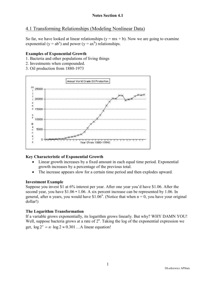
Notes Section 4.1
4.1 Transforming Relationships (Modeling Nonlinear Data)
So far, we have looked at linear relationships (y = mx + b). Now we are going to examine
exponential (y = abx) and power (y = axb) relationships.
Examples of Exponential Growth
1. Bacteria and other populations of living things
2. Investments when compounded.
3. Oil production from 1880-1973
Key Characteristic of Exponential Growth
 Linear growth increases by a fixed amount in each equal time period. Exponential
growth increases by a percentage of the previous total.
 The increase appears slow for a certain time period and then explodes upward.
Investment Example
Suppose you invest $1 at 6% interest per year. After one year you’d have $1.06. After the
second year, you have $1.06 • 1.06. A six percent increase can be represented by 1.06. In
general, after n years, you would have $1.06n. (Notice that when n = 0, you have your original
dollar!)
The Logarithm Transformation
If a variable grows exponentially, its logarithm grows linearly. But why? WHY DAMN YOU!
Well, suppose bacteria grows at a rate of 2n. Taking the log of the exponential expression we
get, log 2 n  n  log 2  0.301 …A linear equation!
1
DLorkiewicz APStats
Notes Section 4.1
Therefore, to transform an exponential scatterplot into a linear scatterplot, take the
logarithm of the response (y) variable and plot with the original explanatory variable.
Note: Real data (like the above graph) will only approximate an exponential curve, so keep in
mind that real data will only give an approximate line when doing the logarithmic
transformation.
But now that we have this line, we can find the least squares residuals after creating the least
squares regression line! Where these residuals lie gives us valuable information on whether
there was a trend of growth or decay during certain periods.
The use of logarithms to obtain a linear pattern from exponential growth complicates
predictions. Remember, the regression line is fitted to the logarithm of the observations. That
means the regression line is predicting the logarithmic values. To get back to the original units,
we must unlog or use the properties if logarithms.
We want to write an exponential function of the form y  a  b x (x & y are variables and a & b
are constants) as a function of the form y  a  bx .
y  a  bx
log y  log  a  b x 
log y  log a  log b x
log y  log a  x  log b
log(variable 1) = constant 1 + (variable 2) (constant 2)
CONCLUSIONS:
1.
If the graph of ( x,log y) is linear, then the graph of (x, y) is exponential.
2.
If the graph of (x, y) is exponential, then the graph of ( x,log y) is linear
Example
The regression line for logarithmic (graph) oil production (example 3) is:
log  yˆ  = -52.686 + (0.02888 • x) where x = year.
So the logarithmic production for 1977 would be: -52.686 + 0.2888 • (1977) = 4.4098.
So to get back to original units (millions of barrels of oil) we do 104.4098 = 25,692.
2
DLorkiewicz APStats
Notes Section 4.1
Log Properties
log b n  n  log b
log m  n  log m  log n
m
log  log m  log n
n
The first rule is very important because the variable in the exponent comes down and yields a
linear equation.
Transforming Power Functions
(We want to write a power function of the form y  ax b as a function of the form y  a  bx .
y  ax b (x & y are variables and a & b are constants)
First take the logarithm of both sides of the function y  ax b
 
log y  log ax b
log y  log a  log x b
log y  log a  b log x
We can rewrite the above equation as a linear equation:
log (variable 1) = (constant 1) + (constant 2) log(variable 2)
or
log y  a  b  log x
So, if the scatter plot of a data set resembles a power function, we can transform it into a linear
scatter plot by taking the logarithm of both variables. log x, log y
3
DLorkiewicz APStats