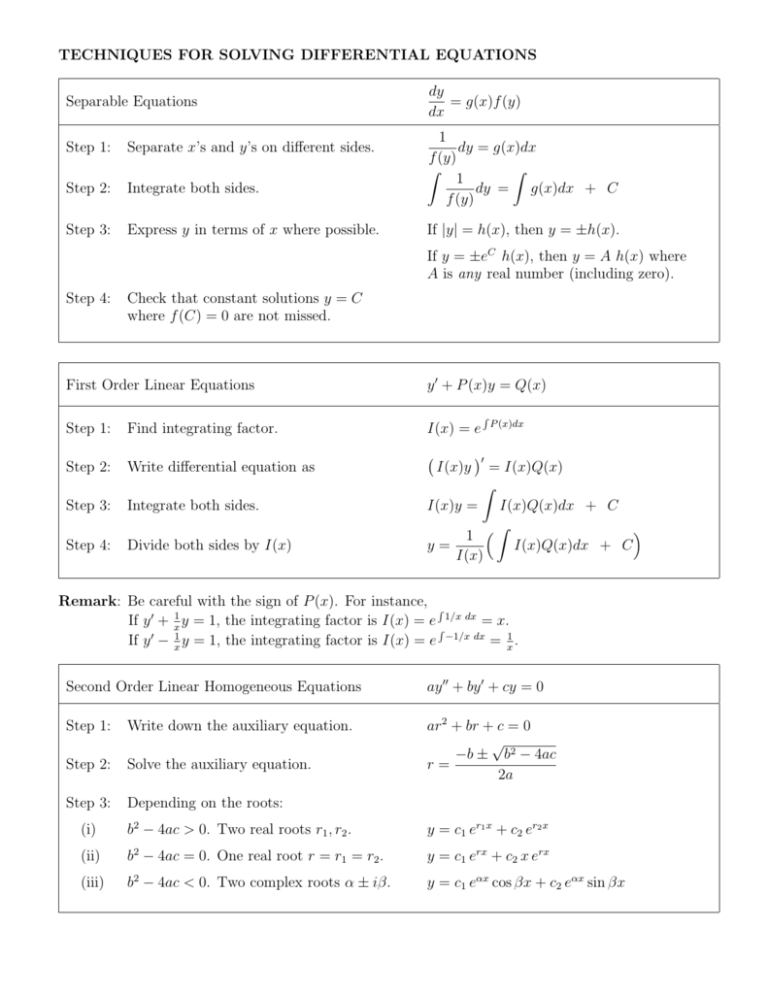
TECHNIQUES FOR SOLVING DIFFERENTIAL EQUATIONS
Separable Equations
Step 1:
Separate x’s and y’s on different sides.
Step 2:
Integrate both sides.
Step 3:
Express y in terms of x where possible.
dy
= g(x)f (y)
dx
1
dy = g(x)dx
f (y)
Z
Z
1
dy = g(x)dx + C
f (y)
If |y| = h(x), then y = ±h(x).
If y = ±eC h(x), then y = A h(x) where
A is any real number (including zero).
Step 4:
Check that constant solutions y = C
where f (C) = 0 are not missed.
First Order Linear Equations
y 0 + P (x)y = Q(x)
Step 1:
Find integrating factor.
I(x) = e
Step 2:
Write differential equation as
Step 3:
Integrate both sides.
Step 4:
Divide both sides by I(x)
= I(x)Q(x)
Z
I(x)y = I(x)Q(x)dx + C
Z
1 I(x)Q(x)dx + C
y=
I(x)
I(x)y
R
P (x)dx
0
Remark: Be careful with the sign of P (x). For instance, R
If y 0 + x1 y = 1, the integrating factor is I(x) = e R 1/x dx = x.
If y 0 − x1 y = 1, the integrating factor is I(x) = e −1/x dx = x1 .
Second Order Linear Homogeneous Equations
ay 00 + by 0 + cy = 0
Step 1:
Write down the auxiliary equation.
Step 2:
Solve the auxiliary equation.
ar2 + br + c = 0
√
−b ± b2 − 4ac
r=
2a
Step 3:
Depending on the roots:
(i)
b2 − 4ac > 0. Two real roots r1 , r2 .
y = c1 er1 x + c2 er2 x
(ii)
b2 − 4ac = 0. One real root r = r1 = r2 .
y = c1 erx + c2 x erx
(iii)
b2 − 4ac < 0. Two complex roots α ± iβ.
y = c1 eαx cos βx + c2 eαx sin βx
Second Order Linear Non-homogeneous Equations
ay 00 + by 0 + cy = G(x)
Method of Undetermined Coefficients
Step 1:
Solve the complementary equation.
ayc00 + byc0 + cyc = 0
yc = c1 y1 (x) + c2 y2 (x)
Step 2:
Write down a trial solution:
(i)
G(x) = P (x)
yp = Q(x)
(i)
G(x) = P (x)ekx
yp = Q(x) ekx
(i)
G(x) = P (x)ekx cos mx or P (x)ekx sin mx
yp = Q(x) ekx cos mx + R(x) ekx sin mx
Here, P (x), Q(x) and R(x) are polynomials of the same degree.
Multiply yp by x (or x2 ) if one of the terms in the sum is y1 (x) or y2 (x).
Step 3:
Substitute yp into the differential equation,
group terms of the same form together,
e.g. xn ekx cos mx, xn ekx sin mx
and solve for the unknown coefficients.
ayp00 + byp0 + cyp = G(x)
Step 4:
Write down the general solution.
y(x) = yc (x) + yp (x)
Second Order Linear Non-homogeneous Equations
ay 00 + by 0 + cy = G(x)
Method of Variation of Parameters
Step 1:
Solve the complementary equation.
ayc00 + byc0 + cyc = 0
yc = c1 y1 + c2 y2
Step 2:
The particular solution has the form:
y p = u1 y 1 + u2 y 2
Write down the two conditions:
Step 3:
Integrate u01 , u02 to get u1 , u2 .
u01 y1 + u02 y2 = 0
u01 y10 + u02 y20 = G(x)/a
G(x)y2
G(x)y1
u01 =
u02 =
0
0
0
a(y1 y2 − y2 y1 )
a(y2 y1 − y10 y2 )
Z
Z
0
u1 = u1 dx + c1
u2 = u02 dx + c2
Step 4:
Write down the general solution.
R
R
y = ( u01 dx + c1 )y1 + ( u02 dx + c2 )y2
Solve the conditions for u01 and u02 .
APPLICATIONS OF DIFFERENTIAL EQUATIONS
ORTHOGONAL
TRAJECTORIES
POPULATION
MODELS
Given family of curves y = f (k, x)
1. Write k in terms of y and x.
2. Differentiate, so k becomes 0.
This is the diff eqn for the curves.
3. Replace y 0 by −1/y 0 . This is the
diff eqn for the orth trajectories.
MIXING PROBLEMS
dy/dx = (rate in) − (rate out)
y is amount of salt at time t.
(rate in) = (vol in) × (conc in)
vol out
×y
(rate out) =
vol at time t
k relative growth rate, K carrying capacity, P0 initial population
Description
Differential Equation
Solution
Eq. Solutions
Natural Growth
dP
= kP, P (0) = P0
dt
P = P0 ekt
P =0
Logistic Model
dP
P
= kP (1 − ), P (0) = P0
dt
K
P =
Predator-Prey
Systems
dR
= kR − aRW
dt
dW
= −rW + bRW
dt
SPRINGS &
ELECTRIC
CIRCUITS
mx00 + kx = 0
P = 0, K
Phase trajectories
(R, W ) = (0, 0)
dW
−rW + bRW
=
dR
kR − aRW
(R, W ) = ( rb , ka )
mx00 + cx0 + kx = F (t)
x displacement
dx/dt velocity
m mass
c damping constant
k spring constant (force/extension)
F (t) external force
Description Differential Equation
Simple
Harmonic
Motion
K
K − P0
, A=
−kt
1 + Ae
P0
LQ00 + RQ0 + Q/C = E(t)
Q charge
dQ/dt = I current
L inductance
R resistance
1/C elastance, C capacitance
E(t) electromotive force
Solution
x(t) = c1 cos ωt + c1 sin ωt = A cos(ωt + δ)
r
q
k
2π
frequency ω =
, period T =
, amplitude A = c21 + c22
m
ω
phase angle δ, cos δ =
c2
c1
, sin δ = −
A
A
√
Damped
Vibrations
mx00 + cx0 + kx = 0
c2 − 4mk
2m
c2 − 4mk > 0 overdamping
x = c1 er1 t + c2 er2 t
2
c − 4mk = 0 critical damping
x = c1 ert + c2 tert
c2 − 4mk < 0 underdamping x = eαt (c1 cos βt + c2 sin βt)
Forced
Vibrations
mx00 + cx0 + kx = F (t)
If F (t) is periodic, then resonance occurs when
the applied frequency ω0 equals the natural frequency ω.
r=
−c ±
KEY
? Definitions • Theorem ◦ Remark ⊗ Extra
9.1 Modeling with Differential Equations
? differential equation, order.
solution, general solution.
? equilibrium solution: a constant solution y = C.
set y 00 = y 0 = 0, y = C in diff eqn and solve for C.
? initial condition, initial value problem.
9.2 Direction Fields and Euler’s Method
? direction field, solution curve.
? autonomous differential equation y 0 = f (y).
if y = g(x) is a solution, so is y = g(x + C).
e.g. natural growth, logistic model
◦ Graphical method:
1. draw direction field.
2. draw solution curve.
◦ Numerical method: Euler’s method, step size h.
Solving y 0 = F (x, y), y(x0 ) = y0 .
1. Set xn = x0 + nh for n ≥ 1.
2. Recursively, yn+1 = yn + hF (xn , yn ) for n ≥ 0.
9.3 Separable Equations
? separable equations, orthogonal trajectories,
mixing problems (see formula sheet)
9.4 Population Models
? logistic differential equation (see formula sheet)
case 1: 0 < P0 < K. P increases and approaches K.
case 2: P0 > K. P decreases and approaches K.
know how to see this from the differential equation.
⊗ natural growth with harvesting
P 0 = kP − c, P (0) = P0
P (t) − kc = (P0 − kc )ekt
trick: subs y = P − kc to get natural growth model.
⊗ logistic model with harvesting (see quiz 11)
P 0 = kP (1 − K
) − c, P (0) = P0
P
q
4c
K
two equilibrium solutions P1 , P2 = 2 1 ± 1 − kK
case 1: P0 < P1 . P approaches −∞
case 2: P1 < P0 < P2 . P increases and approaches P2 .
case 3: P2 < P0 . P decreases and approaches P2 .
trick: subs y = P − P1 to get logistic model.
⊗ Seasonal growth P 0 = kP cos(rt − φ), P = Ce(k/r) sin(rt−φ)
⊗ Seasonal growth with harvesting P 0 = kP cos(rt − φ) − c
⊗ P 0 = kP (1 −
P
)(1
K
−
m
),
P
m extinction level.
9.5 First Order Linear Equations
? first order linear equation (see formula sheet)
◦ to get unique solution from general solution:
initial value problem y(0) = y0
9.6 Predator-Prey Systems
? predator prey equations (see formula sheet)
? phase plane, phase trajectory, phase portrait
◦ know how to derive solutions of natural growth/logistic model
using separation of variables and partial fractions.
? know how to derive, draw and compare
phase trajectories and population graphs
? law of natural growth (see formula sheet)
compare with exponential decay P 0 = −kP
where k is negative, P (t) = P0 e−kt .
⊗
dW
−rW + bRW
Rr W k
=
=⇒ bR aW = C (see S9.6Q7)
dR
kR − aRW
e e
11.1 Second Order Linear Equations
? second order linear equations
P (x)y 00 + Q(x)y 0 + R(x) = 0 homogeneous
P (x)y 00 + Q(x)y 0 + R(x) = G(x) nonhomogeneous
? linear combination, linearly independent solutions
• if differention equation is linear and homoegeneous,
then linear combinations of solutions are solutions.
◦ P (x)y 00 + Q(x)y 0 + R(x) = G(x)
to get unique solution from general solution:
1. initial condition, initial value problem
y(0) = y0 , y 0 (0) = y00
always has unique solution near x = 0
if P, Q, R, G continuous and P (0) 6= 0
2. boundary condition, boundary value problem
y(0) = y0 , y(1) = y1
may not have a solution
? second order linear homogeneous equation,
auxiliary/characteristic equation (see formula sheet)
11.2 Nonhomogeneous Linear Equations
? complimentary equation ay 00 + by 0 + cy = 0
complimentary solution yc (x)
particular solution yp (x)
general solution y(x) = yp (x) + yc (x)
? method of undetermined coefficients (see formula sheet)
? variation of parameters (see formula sheet)
11.3 Applications of Second Order Differential Equations
? spring systems (see formula sheet)
simple harmonic motion
damped vibrations
overdamping (returns to rest slowly)
critical damping (returns to rest fastest)
underdamping (oscillates before coming to rest)
know how to draw graphs of above cases
know how to check if graph cuts x-axis
forced vibrations item[?] electric circuits (see formula sheet)
? steady state solution
is behavior of solution as t → ∞
see S17.3 example 3 note 1
? a function x(t) has period T if x(t + T ) = x(t) for all t.
11.4 Series Solutions
◦ finds solutions near x = 0 because we are writing
the solution as a power series with center x = 0.
P
n
◦ step 1: write y = ∞
n=0 cn x .
step 2: differentiate to get y 0 , y 00 as power series.
step 3: substitute into differential equation. collect terms.
step 4: equate coefficients to get recursion relations.
step 5: solve recursion relations for small n to find patterns.
step 6: write down general solution.
it will be in terms of certain coefficients
e.g. c0 , c1 , which act as arbitrary constants.
step 7: (optional) recognize terms in general solution
as power series of well-known functions.