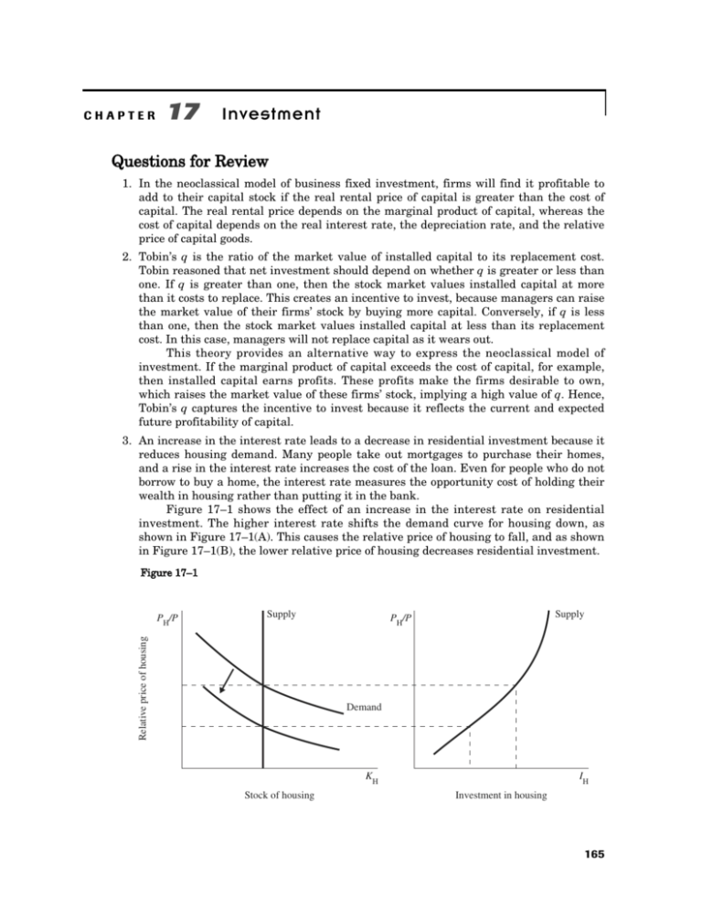
CHAPTER
17
Investment
Questions for Review
1. In the neoclassical model of business fixed investment, firms will find it profitable to
add to their capital stock if the real rental price of capital is greater than the cost of
capital. The real rental price depends on the marginal product of capital, whereas the
cost of capital depends on the real interest rate, the depreciation rate, and the relative
price of capital goods.
2. Tobin’s q is the ratio of the market value of installed capital to its replacement cost.
Tobin reasoned that net investment should depend on whether q is greater or less than
one. If q is greater than one, then the stock market values installed capital at more
than it costs to replace. This creates an incentive to invest, because managers can raise
the market value of their firms’ stock by buying more capital. Conversely, if q is less
than one, then the stock market values installed capital at less than its replacement
cost. In this case, managers will not replace capital as it wears out.
This theory provides an alternative way to express the neoclassical model of
investment. If the marginal product of capital exceeds the cost of capital, for example,
then installed capital earns profits. These profits make the firms desirable to own,
which raises the market value of these firms’ stock, implying a high value of q. Hence,
Tobin’s q captures the incentive to invest because it reflects the current and expected
future profitability of capital.
3. An increase in the interest rate leads to a decrease in residential investment because it
reduces housing demand. Many people take out mortgages to purchase their homes,
and a rise in the interest rate increases the cost of the loan. Even for people who do not
borrow to buy a home, the interest rate measures the opportunity cost of holding their
wealth in housing rather than putting it in the bank.
Figure 17–1 shows the effect of an increase in the interest rate on residential
investment. The higher interest rate shifts the demand curve for housing down, as
shown in Figure 17–1(A). This causes the relative price of housing to fall, and as shown
in Figure 17–1(B), the lower relative price of housing decreases residential investment.
Figure 17–1
Supply
Relative price of housing
PH/P
Supply
PH/P
Demand
KH
Stock of housing
IH
Investment in housing
165
166
Answers to Textbook Questions and Problems
4. Reasons why firms might hold inventories include:
Production smoothing. A firm may hold inventories to smooth the level of produca.
tion over time. Rather than adjust production to match fluctuations in sales, it
may be cheaper to produce goods at a constant rate. Hence, the firm increases
inventories when sales are low and decreases them when sales are high.
Inventories as a factor of production. Holding inventories may allow a firm to
b.
operate more efficiently. For example, a retail store may hold inventories so that it
always has goods available to show customers. A manufacturing firm may hold
inventories of spare parts to reduce the time an assembly line is shut down when
a machine breaks.
Stock-out avoidance. A firm may hold inventories to avoid running out of goods
c.
when sales are unexpectedly high. Firms often have to make production decisions
before knowing how much customers will demand. If demand exceeds production
and there are no inventories, the good will be out of stock for a period, and the
firm will lose sales and profit.
Work in process. Many goods require a number of steps in production and, thered.
fore, take time to produce. When a product is not completely finished, its components are counted as part of a firm’s inventory.
Problems and Applications
1. In answering parts (a) to (c), it is useful to recall the neoclassical investment function:
I = In[MPK – (PK/P)(r + δ)] + δK.
This equation tells us that business fixed investment depends on the marginal product
of capital (MPK), the cost of capital (PK/P)(r + δ), and the amount of depreciation of the
capital stock (δK). Recall also that in equilibrium, the real rental price of capital equals
the marginal product of capital.
a.
The rise in the real interest rate increases the cost of capital(PK/P)(r + δ). Investment declines because firms no longer find it as profitable to add to their capital
stock. Nothing happens immediately to the real rental price of capital, because the
marginal product of capital does not change.
b.
If an earthquake destroys part of the capital stock, then the marginal product of
capital rises because of diminishing marginal product. Hence, the real rental price
of capital increases. Because the MPK rises relative to the cost of capital (which
does not change), firms find it profitable to increase investment.
c.
If an immigration of foreign workers increases the size of the labor force, then the
marginal product of capital and, hence, the real rental price of capital increase.
Because the MPK rises relative to the cost of capital (which does not change),
firms find it profitable to increase investment.
2. Recall the equation for business fixed investment:
I = In[MPK – (PK/P)(r + δ)] + δK.
This equation tells us that business fixed investment depends on the marginal product
of capital, the cost of capital, and the amount of depreciation of the capital stock.
A one-time tax levied on oil reserves does not affect the MPK: the oil companies
must pay the tax no matter how much capital they have. Because neither the benefit of
owning capital (the MPK) nor the cost of capital are changed by the tax, investment
does not change either.
If the firm faces financing constraints, however, then the amount it invests
depends on the amount it currently earns. Because the tax reduces current earnings, it
also reduces investment.
3. a.
There are several reasons why investment might depend on national income.
First, from the neoclassical model of business fixed investment we know that an
Chapter 17
b.
Investment
167
increase in employment increases the marginal product of capital. Hence, if
national income is high because employment increases, then the MPK is high, and
firms have an incentive to invest. Second, if firms face financing constraints, then
an increase in current profits increases the amount that firms are able to invest.
Third, increases in income raise housing demand, which increases the price of
housing and, therefore, the level of residential investment. Fourth, the accelerator
model of inventories implies that when output rises, firms wish to hold more
inventories; this may be because inventories are a factor of production or because
firms wish to avoid stock-outs.
In the Keynesian cross model of Chapter 10, we assumed that I = I. We found the
government-purchases multiplier by considering an increase in government
expenditure of ∆G. The immediate effect is an increase in income of ∆G. This
increase in income causes consumption to rise by MPC × ∆G. This increase in consumption increases expenditure and income once again. This process continues
indefinitely, so the ultimate effect on income is
∆Y = ∆G[1 + mpc + mpc2 + mpc3 + . . . ]
= (1/(1 – MPC))∆G.
Hence, the government spending multiplier we found in Chapter 10 is
∆Y/∆G = 1/(1 – MPC).
Now suppose that investment also depends on income, so that I = I + aY. As
before, an increase in government expenditure by ∆G initially increases income by
³G. This initial increase in income causes consumption to rise MPC × ∆G; now, it
also causes investment to increase by a∆G. This increase in consumption and
investment increases expenditure and income once again. The process continues
until
∆Y = ∆G[1 + (mpc + a) + (mpc + a)2 + (mpc + a)3 + . . . ]
= (1/(1 – MPC – a))∆G.
Hence, the government-purchases multiplier becomes
∆Y/∆G = 1/(1 – MPC – a).
Proceeding the same way, we find that the tax multiplier becomes
∆Y/∆T = – MPC/(1 – MPC – a).
Note that the fiscal-policy multipliers are larger when investment depends
on income.
Answers to Textbook Questions and Problems
c.
The government-purchases multiplier in the Keynesian cross tells us how output
responds to a change in government purchases, for a given interest rate.
Therefore, it tells us how much the IS curve shifts out in response to a change in
government purchases. If investment depends on both income and the interest
rate, then we found in part (b) that the multiplier is larger, so that we know the
IS curve shifts out farther than it does if investment depends on the interest rate
alone. This is shown in Figure 17–2 by the shift from IS1 to IS2.
Figure 17–2
r
LM
Interest rate
168
∆G/(1 – MPC – a)
IS2
IS1
Y
Income, output
From the figure, it is clear that national income and the interest rate
increase. Since income is higher, consumption is higher as well. We cannot tell
whether investment rises or falls: the higher interest rate tends to make investment fall, whereas the higher national income tends to make investment rise.
In the standard model where investment depends only on the interest rate,
an increase in government purchases unambiguously causes investment to fall.
That is, government purchases “crowd out” investment. In this model, an increase
in government purchases might instead increase investment in the short run
through the temporary expansion in Y.
4. A stock market crash implies that the market value of installed capital falls. Tobin’s
q—the ratio of the market value of installed capital to its replacement cost—also falls.
This causes investment and hence aggregate demand to fall.
If the Fed seeks to keep output unchanged, it can offset this aggregate-demand
shock by running an expansionary monetary policy.
5. If managers think the opposition candidate might win, they may postpone some investments that they are considering. If they wait, and the opposition candidate is elected,
then the investment tax credit reduces the cost of their investment. Hence, the campaign promise to implement an investment tax credit next year causes current investment to fall. This fall in investment reduces current aggregate demand and output: the
recession deepens.
Note that this deeper recession makes it more likely that voters vote for the opposition candidate instead of the incumbent, making it more likely that the opposition
candidate wins.
Chapter 17
6. a.
Investment
169
In the 1970s, the baby-boom generation reached adulthood and started forming
their own households. This implies that in our model of residential investment,
demand for housing rose. As shown in Figure 17–3, this causes housing prices and
residential investment to rise.
FiFigure
gure 117–3
7–3
PH/P
PH/P
Relative price of housing
Supply
Demand
Stock of housing
b.
KH
Investment in housing
IH
The Economic Report of the President 1999 (Table B–7) reports that in 1970, the
real price of housing—the ratio of the residential investment deflator to the GDP
deflator—was 27.74/30.48, or 0.91. In 1980, this ratio had risen to 66.62/60.34, or
1.10. Thus, between 1970 and 1980 the real price of housing rose 21 percent. This
finding is consistent with the prediction of our model.
Answers to Textbook Questions and Problems
7. Consider the Solow growth model from Chapters 4 and 5. The Solow model shows that
the saving rate is a key determinant of the steady-state capital stock. If the tax laws
encourage investment in housing but discourage investment in business capital, this
implies that the fraction of output devoted to business investment is lower because of
the tax consequences. Figure 17–4 shows the outcome of the Solow model for low and
high saving rates. At the lower saving rate, business capital-per-worker and business
output-per-worker is also lower. Thus, the tax system distorts the economy’s choice of
business output versus housing.
An alternative way to see this effect is to think of the labor market. With less capital for each worker, the marginal product of labor is lower. Hence, in the long run, the
real wage of workers is lower because of the distortions of the tax system.
Figure 17–4
(n + δ) k
Investment, breakeven investment
170
sH f (k)
sL f (k)
k*L
Business capital per worker
k*H
k